Fully online clustering of evolving data streams into arbitrarily shaped clusters

Elsevier Editorial System(tm) for Information Sciences

Manuscript Draft

Manuscript Number:

Title: Fully Online Clustering of Evolving Data Streams into Arbitrarily Shaped Clusters

Article Type: Full length article Keywords: clustering;

online; evolving;

aribtrary shape; micro-cluster; atmospheric science

Corresponding Author: Mr. Richard William Hyde, BEng(Hons) Corresponding Author's Institution: Lancaster University First Author: Richard William Hyde, BEng(Hons)

Order of Authors: Richard William Hyde, BEng(Hons); Plamen Angelov, PhD; A R MacKenzie, PhD

Suggested Reviewers: Bruno S J Costa PhD [email protected]

Dr Costa is experienced in using online and evolving clustering and classifying techniques and their applications

Feiping Nie

[email protected]

Dr Nie lists research interests in machine learning, online learning, data mining and graph based learning. This paper utilises some graph based techniques.

Gary Fuller

[email protected]

Sample cover letter for submission of a paper to an SPIE journal

Richard Hyde Lancaster University

Intelligent System Lab, B36 Infolab21, South Drive Lancaster University LA1 4WA Professor W Pedrycz

Editor-in-Chief, Information Sciences

Department of Electrical and Computer Engineering, University of Alberta,

9107 - 116 Street, Edmonton, T6G 2V4,

Alberta, Canada 29/01/2016

Dear Professor Pedrycz,

We wish to submit a new manuscript entitled “Fully Online Clustering of Evolving Data Streams into Arbitrarily Shaped Clusters” for consideration by Information Sciences.

We confirm that this work is original and has not been published elsewhere nor is it currently under consideration for publication elsewhere.

In this paper, we report on a new technique for fully online clustering of data into arbitrarily shaped clusters. This is significant because alternative techniques are hybrid online/ offline systems providing incremental updates on the clustering results whereas our technique provide continuous access to the clusters. The paper should be of interest to readers in the areas of mining of data streams or monitoring of online systems in many fields, although our interest lies primarily in atmospheric science.

Please address all correspondence concerning this manuscript to me at [email protected]. Thank you for your consideration of this manuscript.

Sincerely,

Fully Online Clustering of Evolving Data Streams into

Arbitrarily Shaped Clusters

Richard Hyde, Plamen Angelov

Data Science Group, School of Computing and Communications, Lancaster University, Lancaster, LA1 4WA, UK

A R MacKenzie

Birmingham Institute of Forest Research (BIFoR), University of Birmingham, Edgbaston, Birmingham, B15 2TT, UK

Abstract

In recent times there has been an increase in data availability in continuous data streams and clustering of this data has many advantages in data analysis. It is often the case that these data streams are not stationary, but evolve over time, and also that the clusters are not regular shapes but form arbitrary shapes in the data space. Previous techniques for clustering such data streams are either hybrid online / offline methods, windowed offline methods, or find only hyper-elliptical clusters.

In this paper we present a fully online technique for clustering evolving data streams into arbitrary shaped clusters. It is a two stage technique that is accurate, robust to noise, computationally and memory efficient, with a low time penalty as the number of data dimensions increases. The first stage of the technique produces clusters and the second stage combines these micro-clusters into macro-micro-clusters. Dimensional stability and high speed is achieved through keeping the calculations both simple and minimal using hyper-spherical micro-clusters. By maintaining a graph structure, where the micro-clusters are the nodes and the edges are its pairs with intersecting micro-clusters, we minimise the calculations required for macro-cluster maintenance. The micro-clusters themselves are described in such a way that there is no calculation required for the core and shell regions and no separate definition of outer micro-*Manuscript (including abstract)

clusters necessary.

We demonstrate the ability of the proposed technique to join and separate macro-clusters as they evolve in a fully online manner. There are no other fully online techniques that the authors are aware of and so we compare the tech-nique with popular online / offline hybrid alternatives for accuracy, purity and speed. The technique is then applied to real atmospheric science data streams and used to discover short term, long term and seasonal drift and the effects on anomaly detection. As well as having favourable computational characteristics, the technique can add analytic value over hyper-elliptical methods by character-ising the cluster hyper-shape using Euclidean or fractal shape factors. Because the technique records macro-clusters as graphs, further analytic value accrues from characterising the order, degree, and completeness of the cluster-graphs as they evolve over time.

Keywords: online, evolving, clustering, micro-cluster, arbitrary shape

1. Introduction

Recent technological advances in many disciplines have seen an increase in the amount of data being provided in continuous streams of data, i.e. ’on-line data’. These data streams range from machine condition monitoring and atmo-spheric science data to social media analysis. The analysis and clustering of data

5

streams has become increasingly important [1]. However, condition monitoring can suffer from sensor drift due to ageing, temperature fluctuations, modifica-tions or upgrades to machine components, changes in load or type of use. En-vironmental monitoring will also be affected by sensor drift, but also seasonal variations and secular trends due to technological, socio-economic or climate

10

change. While seasonality and other cyclic periodicities can be moved relatively easily off-line, any attempt to do this online renders the analysis vulnerable to aliasing changing seasonal cycles into secular changes. Other problem datasets are short-term but high-dimension and rapidly changing: chemical batch proces-sors [2], environmental mesocosms [3], or ecological manipulation experiments

[4], for instance. Social media analysis will be affected by the inevitable changes in peoples’ taste, population changes and many other influences. In examples such as these the assumption of a stationary data environment is invalid and techniques for data analysis need to be capable of coping with evolving data streams. It is often the case in such data, particularly that incorporating spatial

20

or relational information, that clusters of related data will not be hyper-elliptical and will fall into arbitrarily shaped groupings. The cases for arbitrary shaped clusters are well established and found in many sources [5, 6, 7] . Specifically a case such as that shown in [3] demonstrates the need for evolving clusters of arbitrary shapes - as the nature of the landscape changes over time, so must the

25

clusters.

The ability to adapt our analytic to these secular (non-periodic) changes requires not only a method of reducing the importance of old data but also a way to divide previously singular clusters of data into multiple clusters. With the previously available techniques discussed in section 2 this is achieved, not by

30

dividing the clusters in an online manner, but rather by re-clustering using an offline clustering technique on demand. With ever-increasing data sets, i.e. ’Big Data’, the need to discard or archive the data after processing once becomes necessary for both computational and memory efficiency.

The technique presented in this paper has two distinct stages. The first

35

creates micro-clusters when data samples occur in un-clustered data space. The radius of the micro-clusters,r0, is fixed and should be as small as is practical.

In this newly proposed method we use a simple linear ageing process which reduces the ’Energy’ of a micro-cluster and allows unused micro-clusters to die out completely. Alternative ageing techniques could be used including those

40

exponential types that leave micro-clusters present, with insignificant Energy, but allow them to be ’re-born’ and become relevant in the future with further data. The micro-cluster Energy is renewed every time they receive new data. When no data is received the micro-clusters lose some Energy, gradually fading out. If no data is received for a long time the micro-cluster Energy will reach

45

The second stage searches for overlapping micro-clusters. The micro-clusters are defined as having a kernel region<0.5r0and a shell region>0.5r0. By only

connecting those clusters whose kernel regions overlap into another micro-cluster shell we automatically determine edge micro-micro-clusters. Micro-micro-clusters

50

which do not have at least the user-specified local density, i.e. the minimum number of samples within the radius, remain as separate outlier micro-clusters. Each macro-cluster consists of the graph of intersecting micro-clusters; the ad-jacency relations for each cluster are stored as a property of that micro-cluster. For convenience, we call micro-clusters in adjacency relations (i.e.

in-55

tersecting micro-clusters) Siblings. Those micro-clusters with no Siblings define graphs of order 1 without edges (i.e. intersections) and constitute a macro-cluster graph by themselves. Using this graph structure reduces the calculations required to separate clusters if a cluster dies and breaks a chain graph resulting in two groups of micro-clusters no longer being connected.

60

We call this technique Clustering of Evolving Data-streams into Arbitrary Shapes (CEDAS). We demonstrate the efficacy of CEDAS by testing the algo-rithm for speed and dimensional effects on artificial data sets. Application of CEDAS to the KDDCup99 data stream set is used to compare cluster purity with DenStream and MR-Stream and also to demonstrate the ability of CEDAS

65

to deal with Big Data, adapt to evolving data streams and detect internet in-trusion attacks with high accuracy. We then apply the algorithm to real-world London Air Quality [2] atmospheric monitoring to demonstrate how, by vary-ing the micro-cluster decay time, we can differentiate between short term and long term secular change to discover to discover temporally local anomalies and

70

extremes of the overall distribution.

The rest of the paper is structured as follows: Section 2 provides a review of the current state of the art. Section 3 describes the principles and methodology behind the CEDAS algorithm and provides a description of the pseudo-code given in Appendix A. Section 4 describes the data sets and the methodology of

75

subsections, each with their own discussion. The findings are summarised in section 6 and finally we consider some directions for future work in Section 7.

2. State of the Art

80

Alternative online data stream clustering techniques such as ELM [8], DEC [9] provide online clustering of data streams. Both of these techniques operate on data streams and provide clustering results online but are limited to hyper-ellipsoidal cluster shapes. The basis for ELM is to store the local mean as a cluster centre and to adjust the cluster centre and radii as more data arrives.

85

DEC maintains a list of core and non-core clusters defined by the weight of the cluster. The weight decays over time or is increased as new data samples join the cluster. In this way, core clusters may decay to non-core, non-core clusters my disappear or increase their weight to become core clusters or new, non-core, clusters may be created. In both techniques the clusters that are created are

90

hype-ellipsoidal. In the case of concave cluster shapes DEC may create many smaller hyper-ellipsoidal clusters or one large cluster encapsulating all the data depending on the user parameter values.

Other existing data stream clustering methods such as Chameleon [10], DB-Scan [11] and SPARCL [12] are all techniques for clustering arbitrary shapes

95

offline. Sparcl utilises a two-layer approach whereby k-means [13] clustering is used to create a large number of micro-cluster centres in the first layer. These micro-cluster centres are then further clustered using a hierarchical ap-proach. Chameleon and DBScan are techniques that successfully cluster arbi-trary shapes, however, both work offline and therefore require the full data set.

100

An incremental version of DBScan [14] was proposed which allows for incremen-tal modification of the clusters. However, after each increment the micro-clusters re-built and so require the full data from each increment to be available.

A method known as DenStream was proposed in [14] based on the CluStream [15]. A set of core- and potential-micro-clusters are maintained online. Each

105

decaying the data samples those with a weight below a user-specified threshold are discarded and the memory requirement is limited somewhat although this loses potentially useful micro-clusters. The technique has an initialisation phase, using DBScan, to create an initial set of micro-clusters. Additionally, while the

110

micro-clusters are maintained in an on-line fashion the process of combining the micro-clusters into final clusters is an off-line approach carried out on demand. DenStream is capable of finding arbitrarily shaped clusters as it’s 2nd stage clustering is based on DBScan whereas CluStream, with it’s 2nd stage based on k-means [16], finds hyper-elliptical clusters.

115

Two developments of DenStream known as SDStream [17] and rDenStream [18] improve on the basic DenStream algorithm. SDStream is based on SWClus-tering Algorithm described in [19] and is an offline approach, repeated tempo-rally at incremental time windows. The authors claim improved quality of clus-ters over CluStream [15] however, it remains an incremental offline approach

120

requiring storage of past data. rDenstream is a three stage clustering technique also based on DenStream. In rDenStream any discarded clusters are retained in memory and may be re-introduced to improve the clustering at a later time. Processing of this discarded data requires additional processing time and mem-ory allocation. The 2nd stage of these techniques uses DBScan which has been

125

demonstrated have an order ofD4 _{time penalty, where D is the number of}

di-mensions [20]. DBScan becomes impractical for big data and high didi-mensions and as a result techniques based around DBScan may also suffer from this lim-itation. The combined online-offline approaches limit this time penalty by only applying the offline DBScan macro-clustering function ’on demand’ at reduced

130

frequency.

Grid-based technique MR-Stream [21], divides the data space into a tree of grids of decreasing size (increasing resolution). MR-Stream is a combined on- and offline technique with the cluster grid updated online and regular sec-ond stage clustering of the grid combined with a tree pruning algorithm. In

135

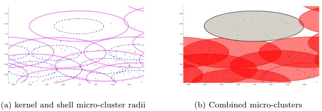
(a) kernel and shell micro-cluster radii (b) Combined micro-clusters

Figure 1: Illustration of kernel micro-cluster regions showing (a) micro-cluster radius in

ma-genta and, micro-cluster kernel radius in blue (b) micro-clusters combined to the

macro-clusters

granularity, or resolution, of the clusters.

A recently introduced technique, CODAS [20] demonstrated a new approach to clustering of continuous data streams into arbitrary shaped clusters. CODAS

140

is a two stage technique with a micro-clustering first stage. The micro-clusters are designated as having an inner ’kernel’ and outer ’shell’ region. This removes the need for classifying micro-clusters as ’edge’ or ’non-edge’ and simplifies the micro-cluster joining calculations. As a result the technique has been demon-strated to be dimensionally stable with a time penalty in the order of D

100), where 145

Dis the number of dimensions. Although CODAS is an online technique it does not allow for the clusters to evolve. That is to say that clusters, once formed, will remain. This means that in cases where the data stream evolves, i.e. forms different clusters at different times, CODAS does not update to remove the old micro-clusters. As a fully online technique, no data is stored and so it is not

150

possible to use techniques such as windowing, or ageing of data to overcome this limitation. The technique presented in this paper builds on the underlying techniques of CODAS but stores the micro-cluster adjacency information to al-low the macro-clusters to evolve and to provide additional information on the structure of the cluster-graph.

3. The Proposed Approach

Traditional offline clustering techniques for arbitrary shapes may categorize data samples as ’core’ or ’non-core’. However, this requires storage of the data samples and ever-increasing storage capacity which is prohibitive for online clus-tering. CEDAS stores only the information related to the micro-clusters and a

160

graph structure recording the micro-cluster connections.

The following terminology is defined for the CEDAS approach:

1. Cluster Graph: the structure that defines which micro-clusters join to form which macro-clusters. This is stored by recording the intersects of each micro-cluster in ’Edge’, together with the appropriate macro-cluster

165

assignation in ’Macro’.

2. Local density: the number of samples per micro-cluster

3. Macro-cluster: a cluster consisting of a number of intersecting micro-clusters.

4. Micro-cluster: a micro-cluster with a local density above the threshold.

170

5. Outlier-micro-cluster: a micro cluster with local density below the thresh-old.

6. Sample: any data point in0n0 dimensions.

7. Threshold: the minimum number of samples within the micro-cluster ra-dius of any sample to form a micro-cluster.

175

In general CEDAS is a data-driven approach to divide the data space in to kernel and shell regions based on a user defined radius,r0. Each micro-cluster

consists of a shell annulus region between radii r0

2 and r0 and a kernel region

being < r0

2. Any micro-cluster above a given density threshold is considered

for macro-cluster membership. Micro-clusters with kernel regions that intersect

180

the threshold but with no intersections are also considered to be macro-clusters. Shell regions are considered to be edges of macro-clusters.

New data from the data stream will fall in to one of 3 regions: 1. empty space, where it will form a new, outlier-micro-cluster

185

2. a micro-cluster shell region, where it will be assigned to the cluster, the cluster count updated and the micro-cluster centre recursively updated to the mean of its samples.

3. a micro-cluster kernel region, where it will be assigned to the micro-cluster and the cluster count updated

190

The micro-cluster that has been modified, or created, by this process is then checked to see if the local density is above the threshold. If this is the case then this micro-cluster is checked for new intersections with other micro-clusters. If new intersections have been made then all the micro-clusters are linked and assigned to the same macro-cluster. This ensures that all linked micro-clusters

195

have the same macro-cluster reference and maintains arbitrarily shaped data space regions of macro-clusters in a fully online manner.

With this approach at any given time a data sample can be checked for its macro-cluster membership, any new sample is immediately clustered and outliers are identified as members of outlier micro-clusters.

200

Figure 1 shows a subset of a plot of test data. Figure 1(a) shows the kernel and shell radii of the micro-clusters. Where the kernel radius of any cluster intersects a shell radius of any other the clusters combine as shown in Figure 1(b). Here the micro-clusters with intersecting kernel and shell regions have combined to form the red shaded cluster region whereas the micro-cluster with

205

the non-intersecting kernel remains separate as the grey region.

3.1. CEDAS Algorithm

This sub-section describes in detail the steps shown in the pseudo-code given in Appendix A. There are 4 distinct steps for the full algorithm including ini-tialisation:

1. Initialization

2. Update Micro-Clusters 3. Kill Clusters

4. Update Cluster Graph

3.1.1. Initialization

215

This creates a structure to store the information related to each micro-cluster and takes place with the first data sample. The ’centre’ and ’radius’ define the region in data space covered by the micro-cluster. ’Count’ stores the total number of data samples that have been allocated to the micro-cluster. The value of ’Count’ is recorded to allow recursive updates to the micro-cluster

220

centre. ’Macro’ is a reference to the macro-cluster to which this micro-cluster belongs. The value of ’Macro’ is the same for all micro-clusters in the ’Sibling’ list. ’Energy’ is a value used to determine the length of time since a micro-cluster received new data. The decay algorithm reduces this value and is discussed later. ’Siblings’ is a list of intersecting micro-clusters, if a micro-cluster has no Sibling

225

list then it is a macro-cluster itself. In graph theory terminology the micro-cluster number paired with each intersect constitutes and ’edge’ of the form {µCc, µCI}, where the first term is the current micro-cluster and the second

term is the intersecting micro-cluster.

3.1.2. Update Cluster

230

This part of the algorithm updates the micro-clusters.

In step 10, a flag is set to record whether any micro-cluster positions are changed or a new micro-cluster is created. If none are changed then the later section of the algorithm that updates the cluster graph is not required to run.

Step 11 finds the distance to the nearest micro-cluster centre. If this distance

235

is less thanr0the new sample is within a micro-cluster and the (Energy) of that

Step 16 checks if the sample is in the micro-cluster kernel region. If not then the micro-cluster centre is updated recursively in step 18 to the mean of all the

240

included samples to date and the indexuof the modified cluster is set. Steps 20-27 create a new micro-cluster if the sample did not lie in any current micro-clusters.

3.1.3. Kill Cluster

Step 28 decays the Energy of each micro-cluster. In the example here we use

245

a simple linear decay but any function could be applied such as the exponential strategy in [14]. Note that with an exponential strategy the Energy of a cluster will never reach zero and some other pruning function will be required. Step 29 lists any clusters that have an Energy less than zero and step 30 checks if any further work is required and returns if no clusters have died.

250

Steps 33-37 remove all dead clusters and also deletes any references to the dead micro-cluster from all the micro-cluster Sibling lists. Micro-clusters are referred to by their index and some may have been removed from the middle of the graph. This means all the references in any Sibling lists that refer to a higher micro-cluster than the one removed must be decremented by 1. This

255

results in an updated cluster graph.

3.1.4. Update Cluster Graph

This section is only required to run if either: 1. a new cluster has been created

2. a cluster centre location has been modified

260

3. a cluster has died and been removed

Step 41 calculates the distance from the updated cluster centre Cu to the

centre of all other micro-clusters Ci. Step 42 checks if the central kernel of

either micro-cluster intersects the other micro-cluster and stores the intersects in the set{j}. Step 43 stores all the new intersects along with all the current

265

number from all the intersecting micro-clusters, Step 45 assigns that number to the modified micro-cluster and step 46 updates the macro-cluster number of the intersecting micro-clusters.

Steps 48-58 reassign the macro-cluster numbers. This is not essential to

270

the algorithm, but without these steps the macro-cluster numbers would be non-consecutive and would increase indefinitely.

4. Test Data

To analyse the performance of the proposed the CEDAS technique the fol-lowing data sets were used:

275

4.1. Spiral High Dimensional Data

This dataset comprises three helical data streams, two of which join mid-way through the test while the other stays separate. These data streams are moved through a range of multiple dimensions to examine the time variance of the analysis with higher dimensional data. The data was analysed using CEDAS

280

with a range of values for Decay and settings of InitialRadius = 0.05 and M inimumClusterSize= 4. The data set is then moved into higher dimensional data space by adding additional dimensional data coordinates. By projecting the data back into 3 dimensions the clustered data can be plotted and the results of cluster membership checked while increasing the complexity of the clustering

285

calculations.

4.2. Mackey-Glass Data Streams

3D data stream consisting of 2 Mackey-Glass time series presented as a data stream. The data streams are solutions of the Mackey-Glass non-linear time delay differential equation [22, 23]. shown in equation 1.

290

dx(t) dt =

ax(t−τ)

1 +x(t−τ)10_−bx(t) (1)

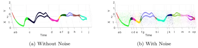
(a) Without Noise (b) With Noise

Figure 2: Illustration of the Mackey-Glass data sets showing a) without noise b) with noise.

The two Mackey-Glass streams are shown in red and green with the noise in blue.

and provide a data stream of 40,020 samples. For each time step 10 random data samples were created around the core value. The data streams are shown in Figure 2a. It can be seen that early in the data the values of both data

295

streams are coincident. They later separate and come together at various times. We would expect that ’recent’ data will produce a changing number of macro-clusters and an online, evolving clustering technique will detect these changes. A further data set was created by adding additional data of random noise samples at every 5th time step creating a dataset of 44,022 samples. This is used to test

300

the robustness of CEDAS to detecting the clusters in a noisy environment. The data can be seen in Figure 2b. By presenting the data sequentially we create a continually evolving data stream rather than a data stream of static values with sporadic variation, such as the KDDCup data set below, which tests the ability of the algorithm to add, merge and separate macro-clusters..

305

The data was presented to the CEDAS algorithm 1 sample at a time to imitate an online data stream and the results plotted at each time step to create a video of the results. The CEDAS algorithm was used to detect and report in the plot title the following information:

1. Definite Clusters: these were defined as clusters containing > 15 data

310

samples and>1 micro-cluster

contained in 1 micro-cluster

3. Last Change: the time period at which the last change in the number of Definite Clusters occurred. This information was recorded to allow the

315

state at that time to be reproduced.

4.3. KDDCup99 Data Stream Set

To further test the CEDAS algorithm in a different environment the KKD-Cup99 [24] dataset was used as a data stream presented to the algorithm se-quentially. The data set consists of approximately 5 million samples in the full

320

data set, 500,000 samples in the 10% reduced set, simulating network intrusion attacks on a military installation. The dataset has 42 features and information to classify the data into 22 attack types in addition to the normal network traffic. This data is used to determine the cluster purity and memory use for compar-ison with alternative techniques and also to validate the clustering results in

325

relation to the number of attack types which occur in a time period.

The dataset is loaded in chunks, to avoid memory issues of holding the data, and passed to the CEDAS algorithm sequentially to mimic an online data stream. To compare the results with alternative techniques the cluster purity is measured at set intervals of 1,000 data samples. The cluster purity

measure-330

ments have also been placed in to groups of 25 to allow direct comparisons to the results in Wan et al [21]. In addition the number of clusters at these time steps is also plotted to compare the number of known attacks within the time period with the number of clusters created by CEDAS.

4.4. London Air Quality Data

335

We then apply the technique to data from the Kings College London Air Quality Website [2]. The data is from one site, Westminster Marylebone, in 2 dimensions, labelledN Ox,P M10. Here and throughout,N Oxis defined as the

reactive oxides of Nitrogen, primarilyN OandN O2, andP M10is defined as the

mass concentration of microscopic airborne particles with aerodynamic diameter

340

of air pollution legislation [25] and to inform the public of adverse air pollution conditions, is captured at 15 minute intervals and ranges from 1stJanuary 2010 to 30th December 2014 for a total of 87,600 samples. This data is used to test CEDAS ability to differentiate short and long term anomalies and follow the

345

temporal drift of real data.

To allow for clustering to take place the data is normalised to a suitable range relative to the micro-cluster radius,r0. Here the range was based on the data available in the dataset and scaled to 0−1. The data had an actual range frommin= 7.200 tomax= 1,447, ppbv (parts-per-billion by volume) forN Ox

350

and min = −0.9, max = 422.8 (µgm−3_{) for P M}

10 and so predicted ranges

of 0 to 1500 and 0 to 200 respectively were used. The scaling introduced by this normalisation has an effect on the local density, joining and separation of micro-clusters and so expert knowledge is required to find suitable values for scientific research involving the cluster results.

355

For this real data test CEDAS was run with different decay times across the different sets of data from London Air Quality kept by Kings College London collected between 2010-2014. The data was presented to the CEDAS algorithm sequentially, inN Ox, P M10 pairs, to mimic on-line data streams. The

micro-clusters were plotted and the transparency of the micro-micro-clusters set according

360

to the value of the Energy in each. In this way if anomalous data appears for a short period of time the cluster adjusts, but it fades over the subsequent time period providing an online visualisation of the Energy of the micro-clusters. This provides a clear visual indication of CEDAS adapting to the changes in the data stream and following long term and short term drift. By using different

365

decay times we demonstrate the different clusters that are created and discuss how this can be useful to investigate different time periods for drift and shift.

5. Results and Discussion

This section contains 3 separate subsections. Within each Subsesction are the results and a discussion of the implication of these results. Subsection 5.1

uses the Mackey-Glass data streams described above to validate the ability of CEDAS to accurately deal with data drift, cluster separation, cluster merg-ing and noise over time. Subsection 5.2 compares CEDAS with alternative techniques CluStream, DenStream and MR-Stream with respect to data dimen-sionality, complexity, processing speed, cluster quality and memory efficiency.

375

Subsection 5.3 applies the CEDAS algorithm to a real data stream from the London Air Quality monitoring system to demonstrate how evolving clustering can aid data mining of data streams containing short term drift, long term drift and short and long term anomalies.

5.1. CEDAS Functionality with Cluster Separation, Cluster Merging, Drift and

380

Noise

To validate the correct functionality of CEDAS the algorithm was applied to the Mackey-Glass data streams usingDecay = 1,000 samples, Radius= 0.05 andM inimumClusterSize= 12.

5.1.1. Cluster Separation and Merging

385

Using the clean Mackey-Glass data stream The sample number at which a change in the number of macro-clusters was detected was stored. After the analysis data was plotted with data from each time period coloured differently. This is shown in Figure 3a.

As expected, after the initial settling period (red), it is seen that at each

390

colour change the number of clusters in the data contained in the preceding decay period has changed. For example, in the green period the data was contained in a single cluster. At the time the colour changes to black, the data in the previous 1,000 samples had just separated to 2 separate clusters. When the colour changes to magenta, the previous 1,000 samples created 1 cluster.

395

5.1.2. The Effects of Noise

(a) Without Noise (b) With Noise

Figure 3: CEDAS Auto Change Detection, changes in colour represent changes in the number

of clusters. The changes detected without noise are also detected with noise with the additional

changes caused by temporary separate micro-clusters before they rejoin the main clusters.

of micro-clusters if the noise falls within them. This increases the likelihood of

400

an initial micro-cluster separating from the main macro-cluster group. If this occurs then the number of macro-clusters may change briefly. This would give the appearance of false positives when compared with the results from dataset without noise. These additional clusters are in fact present at that time and it is accepted that the noise has in fact changed the clustering.

405

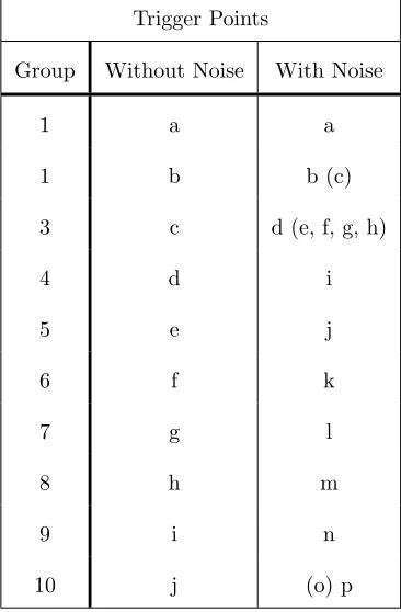
The results are shown in Figures 3a and 3b. In Figure 3b it can be seen that c, e, f, g, h, o are triggered by the noise and could easily be discounted based on he number of samples, if required. The trigger points without noise can be matched to those with noise as shown in table 1. These are discussed in the following sub-sections.

410

5.1.3. False Positives

With any online technique, apparent changes at some point in time may turn out to be irrelevant at a later time. An example of such soon-to-be-irrelevant data anomalies are those that result from the added noise. Rather than calling these ’false positives’, they could be considered as ’temporary or short-term

415

true positives’. In the event these are caused by temporary misplacement of micro-clusters caused by noise, which are rapidly re-absorbed into the macro-cluster, then these addition clusters will have an unusually short lifespan, i.e. considerably shorter than the set decay period. In this way any triggers that are within a user-defined short time span from a previous trigger could be discounted

Table 1: Matching Additional ’Noisy’ Trigger points in brackets with ’No Noise’ trigger points.

Trigger Points

Group Without Noise With Noise

1 a a

1 b b (c)

3 c d (e, f, g, h)

4 d i

5 e j

6 f k

7 g l

8 h m

9 i n

10 j (o) p

if required. However, this is not always desirable, as even short term anomalies may be of interest. They may, for example, indicate the start a general drift in the data.

5.1.4. False Negatives

With appropriate settings for decay time and micro-cluster radius, false

nega-425

tives do not occur. It must be remembered that a different decay time will create different times for cluster separation. This is not indicative of false negatives, but rather a deliberate function of the technique to consider clusters based on data within a defined time frame.

5.1.5. True Positives

430

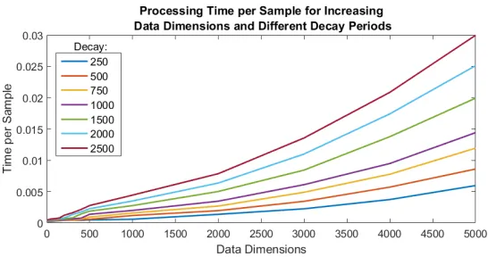
Figure 4: Plot of mean processing time per sample in seconds for varying data dimensionality.

Each line represents the processing time for different decay periods which create a proportional

increase in micro-clusters.

discussed above, CEDAS has successfully detected the same true positives as with the clean dataset as shown in table 1.

5.1.6. True Negatives

435

If we consider the definition of a ’true negative’ to be that ’no changes in macro-clusters are detected when there are none’ then this occurs with every sample that does not create new clusters.

5.2. Comparisons With Alternative Techniques

5.2.1. Speed and Dimensionality

440

By utilising hyper-spheres for micro-clusters the cluster joining technique checking for micro-cluster overlap is much simpler than, e.g. hyper-ellipsoidal micro-clusters. Micro-clusters are joined if the edge of the core hypersphere intersects another hyper-sphere shell. This requires only a comparison between the euclidean distance between cluster centres and the sum of the micro-cluster

445

Figure 5: Comparison of processing time per sample with the decay time. In this example

the decay time is directly proportional to the number of micro-clusters.

With each new data sample being assigned to a single micro-cluster it is

450

only necessary to check the intersections for that micro-cluster and then only if the micro-cluster centre has been modified, or a new micro-cluster has been created. This further reduces the required number of calculations. The radii of the micro-clusters is constant and so we only need to compare the euclidean distance between the changed micro-cluster and all others with 1.5r0.

455

The relationship between the number of data dimensions, decay period and calculation time is plotted in Figure 4. Using Matlab’s curve fitting toolbox the relationship between the data dimensions and time per sample was tested for different decay times. In the case of an evolving data stream with continuous drift the decay time is also proportional to the number of micro-clusters. To

460

investigate the relationship between decay time, and so the number of micro-clusters, and run time the coefficients of the 0x0 term in the linear equations are plotted in Figure 5 and show an approximately linear relationship. This demonstrates that CEDAS has a linear time penalty with both the number of dimensions and the number of micro-clusters.

465

By comparison, Figure 6 shows the relationship between processing time and dimensionality with the same data set for both DenStream [14] and Clustream [15]. We used the Massive Online Analysis [26] implementation running on R3.2.2 in RStudio 0.98.1102 analysing the same spiral high dimensional dataset as for CEDAS. CluStream was also limited to a maximum of 100 micro-clusters.

For both of these techniques, two tests were run using a decay time of 1,000 samples:

1. Both DenStream and CluStream without carrying out the 2nd stage re-clustering until the end of the data stream.

2. We approximated a fully online technique by carrying out the 2nd stage

475

clustering technique at frequent intervals - every 100 samples for Den-Stream and every 10 samples for CluDen-Stream.

For the DenStream 2nd stage re-clustering DBScan [11] was used as imple-mented in the ’R’ package by Hahsler [27] to allow for arbitrary shaped macro-clusters to form in a similar manner to CEDAS. The results shown in Figures

480

6a and 6b are for test 1 and the results shown in Figure 6c and 6d are for test 2. Without 2nd stage re-clustering both DenStream and ClusStream are faster than CEDAS for low dimensionality data. The break even point is approxi-mately 12D for CluStream and 220D for DenStream. When the second stage re-clustering of the micro-clusters is done frequently enough to approximate

485

fully on-line analysis there is significant time penalty for both DenStream and CluStream. In both cases CEDAS is noticeably faster than both DenStream and CluStream and suffers significantly less time penalty for increasing data dimensionality.

5.2.2. Speed and Cluster Quality

490

The KDDCup99 [24] data stream is a popular dataset for testing evolving clustering algorithms such as eClass [28] and it is used here to allow direct comparisons with D-Stream and MR-Stream purity results presented by Wan et al [21]. Two sets of results are presented. The first is the same analysis used by Wan et al. of creating 500 time intervals spaced at 1K samples and placing

495

(a) Without Re-Clustering Low Dimensionality(b) Without Reclustering High Dimensionality

(c) With Re-Clustering, Low Dimensionality (d) With Re-Clustering High Dimensionality

Figure 6: Typical analysis time per sample for DenStream, CluStream and CEDAS across

various dimensional data. a) and b) show CluStream and DenStream without 2nd stage

re-clustering until the end of the data stream. c) and d) show DenStream and CluStream with

It should be noted that purity alone, as defined by equation 2, may be a

500

poor measure by itself.

purity=

Pn

i=1

|Cd i| |Ci|

K ×100% (2)

accuracy=

Pn

i=1 C_id

Pn

i=1|Ci|

×100% (3)

Here Ci is the number of samples in a cluster, CiD is the number of these

samples assigned to the dominant class andNis the number of clusters. In cases where a high number of samples are contained in one cluster with low purity, yet few samples are contained in a high number of clusters with high purity the

505

result is a high mean purity even though most samples are incorrectly assigned. Equally, the reverse is true when few clusters are present, if 99% of the data is correctly assigned in one cluster and two sample are contained in a second, one of which is mis-assigned the mean purity looks poor. In Wan et al. the relevance of this measure is further reduced by taking the mean of these means

510

and so the purity measure is included here for comparison to Wan et al. only and not to attach any particular significance to the result. The cluster accuracy measure as defined in equation 3 is presented in Figure 7d which is a measure of the number of samples that have been correctly assigned to the dominant class. By using both the purity and accuracy measures the quality of the clustering

515

can be stated with greater confidence.

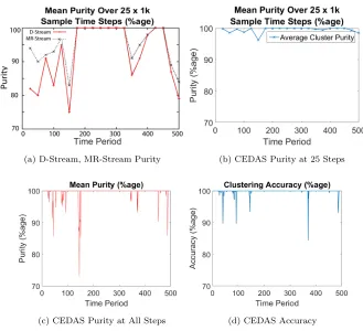
The results of the quality analysis are shown in Figure 7. Although the purity at time period 145 is 73%, the mean over the 25 time periods this is 96%. Using the two time periods selected by Wan et al, 27 and 52, we see that the CEDAS purity was 96% and 99.85% compared with MR-Stream at 97.5% and

520

92% respectively. It is interesting to note that at time periods 26 and 28 CEDAS purity is 100% suggesting that CEDAS adapts quickly to this variation. Using the 25 time periods measure favoured by Wan et al. we see that CEDAS mean purity exceeds that of MR-Stream. When considering the accuracy measure we note that at the time periods 27 and 52 the accuracy measurements are

(a) D-Stream, MR-Stream Purity (b) CEDAS Purity at 25 Steps

(c) CEDAS Purity at All Steps (d) CEDAS Accuracy

Figure 7: (a) Plot of cluster purity (data from Tan et al), (b) Cluster purity for CEDAS by

the same measure as Tan et al. (c) Cluster purity at each time step showing reduced purity.

(d) CEDAS accuracy measure.

98.5% and 99.98% respectively. This indicates that nearly all the samples are correctly assigned to the dominant clusters, but the purity is reduced due to few incorrectly assigned samples in clusters with few members. The accuracy of CEDAS remains close to 100% at all times except for 3 single occasions where it drops to around 90% and 2 at around 95%.

530

Figure 7a shows the results provide by Wan et al. for the mean purity over 25 time steps for both D-Stream and MR-Stream.

Having established via the purity and accuracy measures that the clusters are meaningful it is useful to see if they demonstrate any results of interest. To do this the number of clusters in a time period are compared with the number

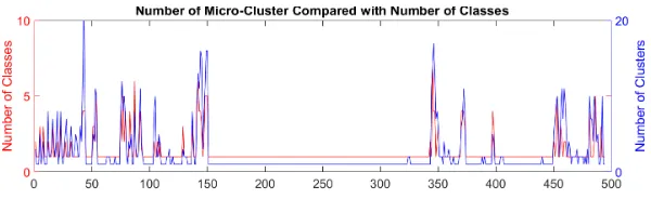
Figure 8: Plot of the number of classes of attack and the number of cluster found by CEDAS

in each time period.

of classes given in the data. The plot of these is given in Figure 8 where it can be seen that each time there is a rise in the number of classes, i.e. attacks, the number of clusters also rises. Given that these clusters have high purity, and the accuracy of clustering is also high, these additional clusters must contain attack vectors unique to each type of attack. There are 50 time periods with attack

540

vectors present and these are detected 100%. As discussed above, occasional separated micro-clusters are a feature of evolving techniques and providing they are short-lived and re-absorbed into the main clusters they can be ignored with reasonable confidence. When the number grows beyond 1 sample per cluster, however, they may be indicative of possible attacks. Thus with a threshold of

545

1 we have 20 false positives. However increasing the threshold to 2 to allow for occasional separated micro-clusters reduces this Figure to 4, and a threshold of 3 reduces this to a single instance. This compares favourably with a mean number of clusters per attack of 8.2.

5.2.3. Memory Efficiency

550

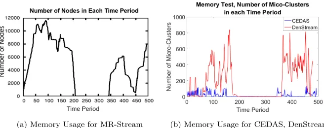
To demonstrate the efficient memory use of CEDAS, we compare the storage required by MR-Stream and DenStream with that required by CEDAS when clustering the KDDCup99 datastream. The results presented by Wan et al. for MR-Stream are shown in Figure 9a and, when the data stream is evolving and has variety, we see that MR-Stream reaches Figures in the thousands of nodes

555

(a) Memory Usage for MR-Stream (b) Memory Usage for CEDAS, DenStream

Figure 9: Plot of the number of nodes or micro-clusters, which equates to memory use, for

MR-Stream, DenStream and CEDAS. CluStream is not shown as it uses a number of

micro-clusters set by the user.

Figure 9b. DenStream has a mean value of 181 and maximum of 839 whereas CEDAS has a mean of 20 and peaks at 137. This demonstrates the significant memory saving of micro-clusters over grid based techniques. Even allowing for

560

the CEDAS cluster description consisting of 5 values there is significant saving over MR-Stream.

5.3. Application to Real Atmospheric Data Streams

This section describes how anomaly detection differs between long-, medium and short-term analysis and how CEDAS copes with such variation. To

demon-565

strate this we are define ’Short Term’ as being 7 days and ’Medium Term’ as being 28 days and ’Long Term’ as being one year. The data used for clustering is N Ox with P M10 from the London Air Quality database for the

Westmin-ster Marylebone monitoring station. Data samples are taken every 15 minutes covering an overall period of 5 years.

570

In Subsection 5.3.1 we consider how the use of a short decay period can reveal short term data drift that would be disguised in medium term decay periods. Subsection 5.3.2 describes the use of medium term decay periods to in-vestigate possible seasonal variations. Finally, in Subsection 5.3.3 demonstrates how medium term decay periods can be used to investigate long term variations.

(a) Processing Speed for MR-Stream (b) Processing Speed for CEDAS

Figure 10: Plots of the processing speed of 9a MR-Stream accumulated time (from [21]) and

9b CEDAS mean time per sample.

In this paper we only provide visual indications of how CEDAS reacts to the evolving data stream. Numerical analysis of the clustering results is discussed in Section 6 Conclusions.

Videos of the CEDAS cluster analysis can be found in the supplementary material.

580

5.3.1. Short Term Drift and Anomalies

Using a decay period equivalent to 7 days of data we can detect the changes in N Ox and P M10 over time. Sample plots are shown in Figure 11 (a)-(c)

showing the cluster analysis at 3 different dates for the preceding 7 days. The data for the preceding 28 day period, for the same dates, is shown in Figures

585

11 (d)-(f).

We can see that the 7 day period preceding 24/03/11 is markedly different from the 7 day period preceding 06/02/11. Despite these difference in the 7 day data, by comparing the plots (d)-(f) we can see that overall, for the preceding 28 day periods the spread of data values has been more consistent. The data

590

(a) Fri 6th (b) Wed 8th (c) Sat 24th

(d) Fri 6th (e) Wed 8th (f) Sat 24th

Figure 11: Sample plots of short term decay periods (a)-(c) and medium term decay periods

(d)-(f). The short term variations indicated in (a)-(c) show the data varies over different 7 day

periods. The medium term variations in (d)-(f) show that the data over the 28 day periods is

more consistent and disguises the 7-day variation.

yellow and magenta cluster of 11 (b) is seen to still be anomalous over the 28 day period, Figure 11 (e), where the clusters are now coloured khaki and blue.

595

This demonstrates that, by selecting suitable decay periods, the clustering results from the proposed algorithm provides relevant analysis of how data be-haves over different time periods and how CEDAS can follow these changes in a fully online manner.

5.3.2. Medium Term Drift and Anomalies

600

The plots in Figure 12 are the cluster results for a 28 day decay period taken at different dates throughout the year. Over the 5 year period of the data streams this approximate pattern is repeated each year. The primary variation is not in the maximum, minimum or range of eitherN Ox orP M10 but rather

in the range of the P M10 : N Ox ratio. This is particularly noticeable when

605

(a) Jan 2011 (b) March 2011

(c) July 2011 (d) Oct 2011

Figure 12: Plots of CEDAS clustering with a 28 day decay time showing variation of the data

over a single year.

P M10 values is greater in March. Anomalous data can still be seen in March

indicating that some unusual events are present.

This demonstrates the ability of CEDAS to follow such seasonal drifts, if they exist, and find data that is anomalous within that local time frame.

610

5.3.3. Long Term Drift and Anomalies

For long term changes, i.e. changes across years, the data could be analysed in multiple ways. For example, the data could be clustered on the full 365 day decay period. However, as we have already indicated in the Subsection 5.3.2 there are variations within that year which may be hidden in the way described

(a) March 2010 (b) March 2012

(c) March 2013 (d) March 2014

Figure 13: Plots of CEDAS clustering with a 28 day decay time showing variation of the data

for March over a 5 year period.

in Subsection 5.3.1. With this information it is reasonable to consider an analysis of 28 day decay periods, at the same date, for subsequent years. Examples of these cluster results are provided in Figure 13 and shows the results for data of the 28 days preceding 01/04 for the years 2010-2015.

The shape of the main cluster can be seen to vary between years indicating

620

the changes in data values. Anomalies are indicated and are for the particular year under consideration. In all cases we see some relatively minor anomalies with values that are slightly different form the main cluster. These could be symptomatic of the data undergoing normal drift and changes. March 2012, however, shows some more extreme anomalies, shown in blue and green, with

particularly high P M10 values. Thus we see that these anomalies detected

in March 2012 were not measured in any other year. This demonstrates how CEDAS may be used to analyse yearly changes, i.e. long term shifts in data and find anomalies independent of drift.

6. Summary and Conclusions

630

A new, fully online clustering technique for clustering data into arbitrarily shaped clusters is proposed. In Section 3 the algorithm has been described. The technique has been applied to the various data sets described in Section 4 and the results presented and discussed. In this section the results are summarised together with appropriate conclusions.

635

6.1. Technique Validity

Section 5.1 demonstrates the ability of CEDAS to accurately divide and merge evolving data streams where appropriate demonstrating the validity of the technique. The proposed algorithm is also shown to be robust to noise.

6.2. Cluster Quality

640

In Section 5.2.2 we compared the proposed algorithm to ClusStream, Den-Stream and MR-Den-Stream and demonstrated that in the tested scenarios CEDAS performed as well as, or better, than all three alternatives. Including the addi-tional accuracy measure provides evidence that the mean cluster purity measure is, in the case of CEDAS, a fair measure of the cluster quality.

645

6.3. Computational Efficiency

When working with stable data-streams with few micro-clusters, DenStream and CluStream approach the speed of the newly proposed technique. However, when the data stream evolves more rapidly, or there are a higher number of micro-clusters, the offline portion of combined online/ offline techniques

be-650

of low dimensionality and where the second stage, offline, technique is not re-quired often then DenStream and CluStream may also be faster. However, this precludes these techniques from being considered as fully online. If excessive periods of time are allowed between second stage clustering important clusters

655

and their information may go unnoticed. By being fully online the proposed technique will not suffer from this limitation. It should also be noted that CluStream finds only hyper-elliptical and not arbitrarily shaped clusters.

6.4. Memory Efficiency

In general, the similarities in the micro-cluster stage means there is a

sim-660

ilarity between memory use for CEDAS, DenStream and ClusStream. The for micro-clusters of a similar size the number will be similar for each technique. MR-Stream is highly memory intensive, not only does it store data for all the cluster nodes, but also for those nodes on the higher plane. MR-Stream claims to use this information to reduce the calculations required for the second stage

665

clustering. However, in the case of a highly populated data space this will re-sults in an increase in memory storage and calculations as a high proportion of the nodes and their parents need to be stored and visited during the second stage clustering. In an effort to reduce the memory requirements MR-Stream prunes nodes with a low density, however this implies a possible loss of data

670

without regard to it’s relevance to the current state.

6.5. Dimensionality

The proposed algorithm has a linear complexity and time penalty relative to the number of data dimensions. DenStream and CluStream have a similar linear complexity and time penalty, however, it is shown in section 5.2 that the

675

penalty is lower for CEDAS. MR-Stream has penalty of nDH _{for dense data}

6.6. Decay Time and the Number of Micro-Clusters

The proposed algorithm has a linear time penalty related to the number of

680

micro-clusters. This is common to all two stage clustering techniques, including those alternatives discussed previously. In cases where the data is fairly static in the data space this has little relevance, however, if the data sample are con-tinuously drifting through the data space there is a direct relationship between the speed of drift and the number of micro-clusters. Thus, in the worst case,

685

there is a linear relationship between the decay time and the processing time. In practice data streams that drift at such a high rate are likely to be rare and may require a different type of analysis in any case. In the case of fairly static data the number of micro-cluster will vary little and no time penalty results from an increase in decay time.

690

6.7. Anomalies, Drift and Time

Sections 5.2.2 and 5.3 discuss the ability of the proposed algorithm to cope with drift and anomaly detection in real data streams. In both these sections CEDAS proved capable of accurately detecting anomalies within the defined time periods demonstrating possible applications in network security and

atmo-695

spheric science research. The results in section 5.2.2 demonstrate how CEDAS could be used to automate detection across multiple dimensions that cannot be easily visualised, whereas Section 5.3 presents a visualization for primary interpretation by the user. In Section 7 some possible techniques are briefly discussed to place a numerical measure of the cluster information.

700

6.8. General Conclusions

Clustering of Evolving Data Streams into Arbitrary Shapes has been demon-strated to be a robust and accurate technique with linear complexity across both data stream size and data stream dimensionality. It is a fully online technique providing constant and immediate access to the clustering results. The

tech-705

7. Future Work

The work presented in this paper demonstrates the ability of the proposed technique to accurately cluster data from evolving data streams, however, no

710

analysis of these clusters is considered. Proposed future work could consider quantitative methods for measuring the clustering results. Well established shape factors such as circularity, solidity or waviness etc may provide insight into the changing relationship between clusters over time. Macro-clusters are agglomerations of micro-clusters which suggests fractal analysis [29]. Providing

715

some measure of the location, spread, size and shape of the macro-clusters can provide information towards a quantitative assessment of the similarity and connection between the internal cluster space and difference measure to other macro-clusters.

Appendix A. Pseudo Code

720

C_iµ - micro-cluster0i0 data structure containing:

C_iµ(Centre) -vector ∈IR with length =number of dimensions, micro-cluster0i0 centre co-ordinates

C_iµ(Count) -integer, number of data samples that have been assigned to micro-cluster0i0

725

C_iµ(M acro) -integer, micro-cluster0i0 macro-cluster membership C_iµ(Energy) -Energy∈IR, current value of assigned to micro-cluster0_i0 C_iµ(Siblings) -vector of integers, list of0Sibling0 micro-clusters linked to micro-cluster0i0

Cµ _{for all the above, but without subscript refers to all micro-clusters}

730

di -∈IR, distances from new data sample to the micro-cluster centrei

{D} - vector of integers, set of indices of dead micro-clusters. (For the decay process described here this is a vector of length 1).

Decay -∈IR, rate at whichC_iµ(Energy) is reduced

735

G- temporary variable for re-assigning macro-cluster numbers i-integer, index value

Nc -integer, number of micro-clusters

r0-∈IR, micro-cluster radius, user input

x-vector∈IR withlength=number of dimensions, current data sample

740

u-integer, index of updated or created micro-cluster

Input: x,R0

Initialization:

1: whilex6={}do

2: if Cµ _{=∅ then}

745

3: C₁µ(Centre) =S

4: C₁µ(Count) = 1

5: C₁µ(M acro) = 1

6: C₁µ(Energy) = 1

7: C₁µ(Sibling) = 1

750

8: Nc=Nc+ 1

9: u=Nc

10: end if

Update Micro-Cluster:

11: u= 0

755

12: dmin=||x−Ciµ(Centre)||min

13: if dmin < r0 then 14: i=argminK

j=1{dj}

16: C_iµ(Count) =C_iµ(Count) + 1

760

17: if di(min)> R₂0 then

18: u=i

19: Cuµ=

(Cµ

u(Count)−1)×Cuµ+S

Cmu u(Count)

20: end if

21: else

765

22: C₁µ(Centre) =x

23: C₁µ(Count) = 1

24: C₁µ(M acro) = 1

25: C₁µ(Energy) = 1

26: C₁µ(Sibling) = 1

770

27: Nc=Nc+ 1

28: end if

Kill Clusters:

29: Ci(Energy) =Ci(Energy)−Decay

30: {D}=f ind(Ci(Energy)<0)

775

31: if {D}=∅ then

32: return

33: else

34: for allDi:

35: deleteC_Dµ i

780

36: deleteC(Sibling) =Di

37: C_iµ(Sibling)> Di=Ci(Sibling)−1

38: Nc=Nc−1

39: end if

40: if u6= 0 then

785

41: dui=||Cuµ(Centre)−C µ

i(Centre)||

42: {j}=f ind(Duj<(1.5×r0))

43: Cµ

u(Sibling) =Cuµ(Sibling)∪ {j}

44: G=min{CCu(Sibling)(M acro)}

45: C_uµ(M acro) =G

46: C_Cµ

u(Sibling)(M acro) =G

47: end if

Housekeeping: Reassign Macro Cluster Numbers

48: Cµ(M acro) = 0 49: G= 0

795

50: fori= 1toNc do

51: if Ci(M acro) = 0then

52: G=G+ 1

53: C_iµ(M acro) =G

54: C_Cµµ i(Sibling)

=G

800

55: else

56: C_Cµµ i(Sibling)

=C_iµ(M acro)

57: end if

58: end for

59: end while

805

Acknowledgment

This work was supported by a NERC studentship through the Coordinated Airborne Studies in the Tropics (CAST) project, grants number NE/J006262/1 and NE/J006181/1.

The authors would like to thank Dr. Gary Fuller for his help selecting data

810

from the London Air Quality Dataset.

The second author would like to acknowledge the partial support through The Royal Society grant IE141329/2014 “Novel Machine Learning Paradigms to address Big Data Stream”

References

815

pages (2002-19) (2002) 1. doi:10.1145/543614.543615.

URLhttp://portal.acm.org/citation.cfm?doid=543613.543615

820

[2] London Air Quality Network :: Welcome to the London Air Quality Net-work Data Downloads.

URLhttp://www.londonair.org.uk/london/asp/datadownload.asp

[3] K. P. Wyche, P. S. Monks, K. L. Smallbone, J. F. Hamilton, M. R. Alfarra, a. R. Rickard, G. B. McFiggans, M. E. Jenkin, W. J. Bloss, a. C. Ryan,

825

C. N. Hewitt, a. R. MacKenzie, Mapping gas-phase organic reactivity and concomitant secondary organic aerosol formation: chemometric dimension reduction techniques for the deconvolution of complex atmospheric data sets, Atmospheric Chemistry and Physics 15 (14) (2015) 8077–8100. doi: 10.5194/acp-15-8077-2015.

830

URLhttp://www.atmos-chem-phys.net/15/8077/2015/

[4] R. J. Norby, M. G. De Kauwe, T. F. Domingues, R. A. Duursma, D. S. Ellsworth, D. S. Goll, D. M. Lapola, K. A. Luus, A. R. MacKenzie, B. E. Medlyn, R. Pavlick, A. Rammig, B. Smith, R. Thomas, K. Thonicke, A. P. Walker, X. Yang, S. Zaehle, Model-data synthesis for the next generation of

835

forest free-air CO2 enrichment (FACE) experiments., The New phytologist 209 (1) (2015) 17–28. doi:10.1111/nph.13593.

URLhttp://www.ncbi.nlm.nih.gov/pubmed/26249015

[5] V. Chaoji, Efficient Algorithms for Mining Arbitrary, Ph.D. thesis, Rens-selaer Polytechnic Institute (2009).

840

URL _{http://www.cs.rpi.edu/{~}zaki/PaperDir/PhdTheses/chaoji.}

pdf

[6] C. P¨oelitz, G. Andrienko, N. Andrienko, Finding arbitrary shaped clusters with related extents in space and time, EuroVAST 2010: International Symposium on Visual Analytics Science and Technology (2010) 19–25.

845

019-025.pdf.abstract.pdf;internal{&}action=action.

digitallibrary.ShowPaperAbstract

[7] K. Partington, J. Cardille, Uncovering Dominant Land-Cover Patterns of Quebec: Representative Landscapes, Spatial Clusters, and Fences, Land

850

2 (4) (2013) 756–773. doi:10.3390/land2040756. URLhttp://www.mdpi.com/2073-445X/2/4/756/htm

[8] R. Dutta Baruah, P. Angelov, Evolving local means method for clustering of streaming data, IEEE International Conference on Fuzzy Systems (2012) 10–15doi:10.1109/FUZZ-IEEE.2012.6251366.

855

[9] R. D. Baruah, P. Angelov, DEC: Dynamically evolving clustering and its application to structure identification of evolving fuzzy model, Transaction on Cybernetics 44 (9) (2013) 1–16. doi:10.1109/TCYB.2013.2291234. [10] G. Karypis, E.-H. Han, V. Kumar, Chameleon: hierarchical clustering using

dynamic modeling, Computer 32 (1999) 68–75. doi:10.1109/2.781637.

860

[11] M. Ester, H. P. Kriegel, J. Sander, X. Xu, A density-based algorithm for discovering clusters in large spatial databases with noise, Second Interna-tional Conference on Knowledge Discovery and Data Mining (1996) 226– 231doi:10.1.1.71.1980.

URL http://citeseerx.ist.psu.edu/viewdoc/summary?doi=10.1.1.

865

20.2930

[12] V. Chaoji, M. Al Hasan, S. Salem, M. J. Zaki, SPARCL: Efficient and effec-tive shape-based clustering, Proceedings - IEEE International Conference on Data Mining, ICDM (2008) 93–102doi:10.1109/ICDM.2008.73. [13] J. B. MacQueen, Kmeans some methods for classification and

analy-870

sis of multivariate observations, 5th Berkeley Symposium on Mathe-matical Statistics and Probability 1967 1 (233) (1967) 281–297. doi: citeulike-article-id:6083430.

[14] F. Cao, M. Ester, W. Qian, A. Zhou, Density-based clustering over an

875

evolving data stream with noise, in: . . . Conference on Data Mining, no. 2, 2006, pp. 328–339. doi:10.1145/1552303.1552307.

[15] C. C. Aggarwal, T. J. Watson, R. Ctr, J. Han, J. Wang, P. S. Yu, A framework for clustering evolving data streams, Proceedings of the 29th international conference on Very large data bases (2003) 81–92doi:

880

10.1.1.13.8650.

URL http://citeseerx.ist.psu.edu/viewdoc/summary?doi=10.1.1. 13.8650

[16] J. A. Hartigan, M. A. Wong, Algorithm AS 136: A K-Means clustering algorithm, Applied Statistics 28 (1) (1979) 100. doi:10.2307/2346830.

885

URL http://www.jstor.org/stable/10.2307/2346830?origin=

crossref

[17] J. Ren, R. Ma, Density-based data streams clustering over sliding windows, in: 2009 Sixth International Conference on Fuzzy Systems and Knowledge Discovery, Vol. 5, IEEE, 2009, pp. 248–252. doi:10.1109/FSKD.2009.553.

890

URL http://ieeexplore.ieee.org/lpdocs/epic03/wrapper.htm? arnumber=5360620

[18] L.-x. Liu, Y.-f. Guo, J. Kang, H. Huang, A three-step clustering algorithm over an evolving data stream, 2009 IEEE International Conference on Intelligent Computing and Intelligent Systems (2009)

895

160–164doi:10.1109/ICICISYS.2009.5357749.

URL http://ieeexplore.ieee.org/lpdocs/epic03/wrapper.htm? arnumber=5357749

[19] A. Zhou, F. Cao, W. Qian, C. Jin, Tracking clusters in evolving data streams over sliding windows, Knowledge and Information Systems 15 (2)

900

(2008) 181–214. doi:10.1007/s10115-007-0070-x.

[20] R. Hyde, P. Angelov, A new online clustering approach for data in arbitrary shaped clusters, in: 2015 IEEE 2nd International Con-ference on Cybernetics (CYBCONF), IEEE, 2015, pp. 228–233.

905

doi:10.1109/CYBConf.2015.7175937.

URL http://ieeexplore.ieee.org/lpdocs/epic03/wrapper.htm? arnumber=7175937

[21] L. Wan, W. K. Ng, X. H. Dang, P. S. Yu, K. Zhang, Density-based cluster-ing of data streams at multiple resolutions, ACM Transactions on

Knowl-910

edge Discovery from Data 3 (3) (2009) 1–28. doi:10.1145/1552303. 1552307.

URLhttp://portal.acm.org/citation.cfm?doid=1552303.1552307

[22] M. Mackey, L. Glass, Oscillation and chaos in physiological control systems, Science 197 (4300) (1977) 287–289. doi:10.1126/science.267326.

915

URLhttp://www.sciencemag.org/content/197/4300/287.short

[23] L. Glass, M. Mackey, Mackey-Glass equation, Scholarpedia 5 (3) (2010) 6908. doi:10.4249/scholarpedia.6908.

URL http://www.scholarpedia.org/article/

Mackey-Glass{_}equation

920

[24] K. C. 1999, KDDCup 1999, Tech. rep. (1999).

URL http://kdd.ics.uci.edu/databases/kddcup99/kddcup.

data{_}10{_}percent.gz

[25] PCC, 2012 Air quality updating and screening assessment, Tech. Rep. April, Plymouth City Council, Plymouth (2012).

925

URL http://www.plymouth.gov.uk/air_quality_updating_

screening_assessment_2012.pdf

[26] A. Bifet, G. Holmes, B. Pfahringer, P. Kranen, H. Kremer, T. Jansen, T. Seidl, MOA: Massive online analysis, a framework for stream classifica-tion and clustering, HaCDAIS 2010 11 (2010) 3.

930

[27] M. Hahsler, Density based clustering of applications with noise (DBSCAN) and related algorithms. (2015).

URLhttp://cran.r-project.org/package=dbscan

[28] P. Angelov, X. Zhou, Evolving fuzzy-rule based classifiers from data

935

streams, IEEE Transactions on Fuzzy Systems 16 (6) (2008) 1462–1474.

doi:10.1109/TFUZZ.2008.925904.

[29] R. Botet, R. Jullien, M. Kolb, Hierarchical model for irreversible kinetic cluster formation, Physics A: Mathematical and General 17 (2) (1984) 75– 79. doi:10.1088/0305-4470/17/2/009.

Figure

Figure

Rob MacKenzie has expertise in

computer simulation of atmospheric aerosol

and the

effects of

vegetation on atmospheric composition

. His work on urban sustainability more broadly includes

interdisciplinary tools for assessing resilience that have been applied in Birmingham, Lancaster,

London, and Milan, presented in Designing Resilient Cities, and further developed through the

University of Birmingham Policy Commission on Future Urban Living

.

Rob has also carried responsibility for major research infrastructure throughout his career: the

Geophysica high-altitude research aircraft (1996-2010) and, since November 2013, the inaugural

Director of the

Birmingham Institute of Forest Research

. BIFoR is initiating a >£10m Free-Air Carbon

dioxide Enrichment (FACE) facility, one of 4 parts of a uniquely ambitious global research platform

for the study of the resilience of forests under environmental change.

Figure

Supplementary material for on-line publication only

Supplementary material for on-line publication only

Supplementary material for on-line publication only