A neural network filtering approach for similarity based remaining useful life estimation

https://doi.org/10.1007/s00170-018-2874-0

ORIGINAL ARTICLE

A neural network filtering approach for similarity-based remaining

useful life estimation

Oguz Bektas1·Jeffrey A. Jones1·Shankar Sankararaman2·Indranil Roychoudhury3·Kai Goebel4,5

Received: 22 March 2018 / Accepted: 8 October 2018 ©The Author(s) 2018

Abstract

The role of prognostics and health management is ever more prevalent with advanced techniques of estimation methods. However, data processing and remaining useful life prediction algorithms are often very different. Some difficulties in accurate prediction can be tackled by redefining raw data parameters into more meaningful and comprehensive health level indicators that will then provide performance information. Proper data processing has a significant importance on remaining useful life predictions, for example, to deal with data limitations or/and multi-regime operating conditions. The framework proposed in this paper considers a similarity-based prognostic algorithm that is fed by the use of data normalisation and filtering methods for operational trajectories of complex systems. This is combined with a data-driven prognostic technique based on feed-forward neural networks with multi-regime normalisation. In particular, the paper takes a close look at how pre-processing methods affect algorithm performance. The work presented herein shows a conceptual prognostic framework that overcomes challenges presented by short-term test datasets and that increases the prediction performance with regards to prognostic metrics.

Keywords Similarity-based RUL calculation·C-MAPPS datasets·Neural networks·Data-driven prognostics

Part of this work was completed while Oguz Bektas was an exchange visitor at the Universities Space Research Association at NASA Ames Research Center, whose kind hospitality is gratefully acknowledged.

Shankar Sankararaman performed this work while being employed at SGT Inc., NASA Ames Research Center, Moffett Field, CA 94035, USA.

Oguz Bektas

o.bektas@warwick.ac.uk

Jeffrey A. Jones

J.A.Jones@warwick.ac.uk

Shankar Sankararaman

shankar.sankararaman@pwc.com

Indranil Roychoudhury

indranil.roychoudhury@nasa.gov

Kai Goebel

kai.goebel@nasa.gov

1 _{Warwick Manufacturing Group, University of Warwick,}

Coventry CV4 7AL, UK

1 Introduction

Prognostics is a promising technology which enables to manage assets based on their remaining useful life (RUL) and future health conditions [1,2]. The potential of prog-nostics relies on its capacity to anticipate the evolution of anomalous conditions in time. It seeks to provide enough time for maintenance operation and sets off the alarm for necessary actions. A key feature in prognostics is to accu-rately predict the RUL of systems whose current condition and historical data are available. Such data-driven prognos-tics makes use of historical condition monitoring informa-tion for analysing and modelling of desired system output [1]. Most of these data-driven approaches originated from

2 _{Data Science and Analytics Manager, Pricewaterhouse}

Cooper, San Jose, CA 95110, USA

3 _{Stinger Ghaffarian Technologies, Inc., NASA Ames Research}

Center, Moffett Field, CA 94035, USA

4 _{NASA Ames Research Center, Moffett Field, CA 94035, USA}

5 _{Division of Operation and Maintenance Engineering, Lule˚a}

“conventional numerical” methods and “machine learning” applications [3].

The common conventional methods include regression models [4,5], Wiener processes [6], wavelets [7,8], hidden Markov model [9, 10], Kalman filters [11, 12], particle filters [13,14] and the Gaussian process [15]. A widespread range of conventional applications dealing with different domains can be found in the literature, such as fatigue degradation evolution in materials [16], ageing of batteries, [17], fault detection and isolation of mechatronic systems [18–22], and failure of electronic components [23].

When a data-driven model is planned and tested, it has to face the challenges brought up by the complexity of real-world systems [24]. In general, these include dealing with incomplete knowledge of future load conditions, inaccurate estimation of the current state of health, poor evolution mod-els, sensor noise and varying operating conditions. In con-ventional methods, the selection of a prognostic algorithm for complex systems depends on an understanding of the challenges associated with the type of systems [25]. There-fore, it is not surprising that most prognostic research work to date has been theoretical and restricted to a small num-ber of models, and there have been few published examples of prognostic applications being fully fielded in condition monitoring of complex systems that are exposed to a range of operating conditions [26].

Indeed, prognostics of complex engineered systems remains an area of active research and development. Increasing trends appeared in the prognostic field have been summarised in the literature [27–31]. Machine learn-ing methods and related techniques can offer an impor-tant part of the solution [3]. They can be used when an explicit degradation model is not available, but suffi-cient condition monitoring data have been collected. Arti-ficial neural networks are the most common machine learning methods used in prognostic applications [32–34]; other methods include decision trees [35], support vec-tor machines [36–38], case-based reasoning [39], cluster-ing [40], classification [41], Bayesian methods [42, 43] and Fuzzy logic [44, 45]. Such approaches make use of historical data for estimating the health conditions rather than building models based on physical system characteristics.

A core issue encountered in making meaningful RUL estimations is to account for different kinds of uncertainties from various sources in the whole exercise such as process noise, measurement noise, and inaccurate process models [1]. Particularly, uncertainties arising from complex systems make identification of their source even harder. Complex systems are formed of various interacting components in which the collective actions are difficult to deduce from those of the individual elements, predictability is limited and responses do not scale linearly [46]. In this respect, among

the data-driven approaches, the artificial neural networks (ANNs) have been the most used methods to prognostics, due to their capability of approximating non-linear complex functions [1].

Condition monitoring of the complex systems is usually based on multiple sensors that receive information on the system health and recognise any potential failures at an early stage so that corrective actions can be suggested in a timely manner. However, evaluation of sensor data from various components is often a challenge due to complicated interdependencies between measured data and actual system conditions [47].

As a function of operating conditions, complex systems work at superimposed operational margins at any given time instant. The wear process of such systems is not deterministic, and usually not one-dimensional [48]. The multidimensional and noisy data stream is monitored from a large number of channels (such as use or environmental conditions, direct and indirect measurements which are potentially related to damage) from a population of similar components [49]. Therefore, a simple analytical model is unable to present the wear phenomena and one should consider the decision-making process in multidimensional condition monitoring case [50]. In such cases, a well-known pre-processing step is to perform component-wise normalisation to provide a common scale across all the features of condition monitoring data [51].

While the importance of multidimensional data and the multiple axes of information have been recognised in the literature, there is still a gap in analysis of such data, leaving the analysts with yet more information to process through the complex systems [52]. This can be attributed to an incomplete understanding of the multidimensional failure mechanisms and lack of correlation between different but similar data sources.

The review of literature in this section shows that, due to the incomplete understanding on the multidimensional failure mechanisms and lack of support between data sources, current methods lack the ability to deal effectively with complicated interdependency [47], multidimensional data [48] and noisy data [49]. Further conventional pre-processing is unable to deal with this efficiently. Moreover, emerging technologies for the Internet of Things (IoT) still face some enormous challenges on data security and confidentiality [53].

data integrity, as well as dimensionality reduction and RUL estimation.

In the work shown here, a component-wise normalisation method is first used to standardise multidimensional data for a better understanding of the multidimensional failure mechanisms. Then, a neural network function is trained to map between a dataset of numeric inputs (multidimensional raw data) and a set of numeric targets (normalised data). The network function here is a kind of dynamic filtering, in which one can fit multidimensional mapping problems well. These two data processing steps play an important role in modelling performance health indicators for prognosis. A similarity-based remaining useful life estimation model identifies the best matching portion of training health indicators for each test health indicator and produces future multistep predictions of system wear levels.

The method is evaluated by “final test” subset of PHM08 data challenge from NASA Prognostics Center of Excellence data repository. Results demonstrate that performance deterioration of initially trained subsets can be used to successfully predict RULs of test subsets.

The developed prognostic model is based on the fun-damental notions of the prognostics such as the degrada-tion over time, monotonic damage accumuladegrada-tion, detec-table ageing symptoms and the correlation of these symp-toms with RUL [49]. With consideration of these, this work has the objectives to investigate data filtering and processing techniques as well as remaining useful life predictions.

2 Background and motivation

As prognostic technology advances to maturation in real-life applications, the desire for using data-driven processing methods has considerably risen. Data-driven prognostic approaches are used for modelling of the desired system output where historical condition data are available [54]. However, the issue of output assignment arises when a set of trajectories with different initial wear levels and multi-regime operating conditions is inserted into the same data-driven filtering model. This is the case in some common datasets such as the C-MAPSS datasets (of which the PHM08 dataset is a part) [55].

Ensuring performance and safety in complicated and safety-critical systems is a major issue, and in particular, complexity is of the most prominent problems that must be tackled to make theoretical frameworks applicable to real industrial applications [56]. The main motivation of this paper is to provide an adaptive model for remaining useful life estimations on multidimensional condition monitoring data. Multidimensional data are defined in terms of dimen-sions, which are organised in dimension hierarchies [57]. To model the multidimensional space, letbe the space of

all dimensions. Operational trajectory,T, in this space is a set of time,t, operating conditions (or regimes),r, and the condition monitoring data,x.

T(i)= ti,ri,xi, i=1,2,· · ·, n,and,T,t,r,x,∈

(1)

wheretfollows a sequential order (and each variable oftis unique), andrcan only have certain values. In other words, the unique values of the operating conditions vector, “θ (r)”, are limited to the number of regimes, “np”.

θ (r)= {ri}i{1,2,3,···,n},where, r=(r1, r2, r3· · ·rn) (2)

θ (r)=(1,2,· · ·, np) (3) Considering that the sensors working at different operating conditions provide similar readings with those in the same regime, the vector,x=(x1, x2, x3,· · ·xn), would

align in certain domains,ϑri, which are bounded by lower

lriand upper limitsuri.

ϑri=(lri, uri)⇒

xi∈:lri ≤xi≤uri)

, (4)

i=(1,2,· · ·n) and ∀ri, ri∈θ (r)=(1,2,· · ·, np) (5)

Figure1shows a sample of multidimensional trajectory (the data are taken from the PHM08 dataset). The sensor readings represent various operating conditions and condition monitoring measurements which, for this dataset, falls into six cluster domains (ϑ).

To produce meaningful information from such a trajec-tory, Wang et al. and Peel [51,58] proposed a component-wise “multi-regime normalisation” method to standardise the sensor readings according to each other within the same domain. In these cases, the normalisation is applied into the PHM08 dataset which is formed of multiple trajectories with distinct health levels that can be found in the condi-tion monitoring data. The health levels in these trajectories evolve with exponential characteristics [48].

h(t)=1−d˚−expat˚ b˚ (6)

where ˚d is an arbitrary point in the wear-space (the trajectories are observed with some non-zero initial wear degradation), ˚a and ˚b are the model parameters. In this scenario, each trajectory in the dataset starts at a distinct point and follows a characteristic “h” pattern. Considering the multiple trajectories, the entire dataset with its all components needs to be standardised together to preserve the characteristic wear levels. For the case considered in the works of Wang et al. and Peel [51,58], all trajectories were available at the same time. The “normalisation at once” has therefore not been a major issue. Nevertheless, it would be rather unlikely to find such data in a real-life scenario due to the restrictions on data proprietary considerations and confidentiality [59]. In a real-world scenario, the “multi-regime normalisation” should be repeated for each novel incoming trajectory in order to calculate the changed population characteristics such ashandd.

Heimes [32] provided a “neural network filtering” approach that can be an alternative to the “multi-regime normalisation” . Unlike the regime normalisation methods, a trained neural network function can filter the necessary degradation information. ANNs are computational algo-rithms loosely inspired by the observed behaviour of biolog-ical neural networks of the brain, and they are compromised of data processing neurons [60]. The networks form a set of interconnected functional relationships between many input series and a desired unique output where the relationship can be trained for optimal performance [11]. Since an oper-ational trajectory of a complex system is formed of multiple sensor observations, there are multiple corresponding val-ues at each time point which can be used to train network function with multi-input series.

x =[x1, x2, x3,· · ·, xt,· · ·, xn] (7)

xt =xt,1, xt,2, xt,3,· · ·xt,ns

(8)

The basic method for supervised neural networks is to train a non-linear model using data representing the cases of interest by reducing measurable errors through a regularisation algorithm. In certain complex engineering applications, the observations from the system may not be precise, and the desired exact results may not have a direct mathematical link with the input data. An ANN is a convenient tool for modelling such a system without knowing the exact relationship between input,x, and output data series,y[61].

y=fN N(x) (9)

However, the supervised learning task of inferring an ANN function from “labelled historical condition data” carries the potential risk of failing to identify population characteristic, wear levels (“d”) and “h” pattern. Without accurately specifying the initial wear levels and “h” pattern,

the network filtering may be thrown off since the initial bias may dictate the sensitivity to RUL estimation.

By considering both component-wise multi-regime nor-malisation methods proposed by Wang et al. and Peel [51,58] and the neural network filtering model of Heimes [32], an initial unsupervised learning task that learns hid-den degradation behaviour can be used. In other words, the initial wear levels can be identified as desired, and the

“normalisation at once” issue can be solved by a neural

network-based supervised learning data filtering method. Then, the remaining useful life of a test sample can be predicted by using the actual lifetime of similar examples so that the final prediction of RUL can be collaboratively estimated from multiple historical instances. The novelty presented in this paper is to perform the output parame-ters assignment (unsupervised learning) and data filtering (supervised learning) steps sequentially.

The proposed model combines the work of “multi-regime normalisation” [51,58] with the work of a neural network filtering approach ([32]), so that normalised trajectories can form an output,y for the network filtering. The main hypothesis for this theory is that there is the possibility that, after applying normalisation for a certain number of trajectories, novel data can be filtered independently. Following this hypothesis, it is also expected that the new model will be more effective for the similarity-based remaining useful life estimations.

3 Experimental data

To start the acquisition of condition monitoring information for effective prognostic applications, the first major issue is to find available data sources. A common database is an important instrument for understanding the problems and developing the methodologies. If such a database includes information from several relevant operational domains, it can form the basis for data acquisition and required actions [62]. Application of the common database practice also allows for the comparison of current activities and potential fields of improvement with regard to other methods in the literature [63].

One of the most applied datasets in the literature is the C-MAPSS datasets. Commercial Modular Aero-Propulsion System Simulation (C-MAPSS) was developed by NASA to simulate realistic large commercial turbofan engines [48,

64]. The software is coded in Matlab and Simulink (The MathWorks, Inc.) environments with some editable input parameters that allow the developers to enter specific values of their choice regarding operational profile, environmental conditions, etc [64].

Degradation Simulations [55]. Trajectories differ from each other and were simulated under various combinations of operational conditions, regimes and fault modes. The datasets have been made publicly available for training and validation of results [55].

The features of C-MAPSS engine degradation sim-ulations include the following characteristics that make them practical and suitable for developing prognostic algo-rithms on multistep ahead remaining useful life calcu-lations [55,59].

– Each dataset contains multiple multidimensional time series representing sensor magnitudes over time and three operational settings that indicate variations of operational regimes.

– The sensors are contaminated with high levels of noise that simulate the variability of parameter readings dur-ing operations. There is also very little system informa-tion and no sensor labels available to developers. – Each trajectory has a distinct degree of an initial wear

level and manufacturing variation. This wear level is considered normal, and it is unknown to the users. – The fault signature is “hidden” on account of

opera-tional conditions and noise.

– Datasets are divided into training and test trajectories (individual subsets). The training trajectories are implemented to build up to train remaining useful life prediction algorithms, and therefore, the instances are formed of complete run-to-failure data which can be used to feed the test trajectories that are only set up by shorter instances up to a certain time prior to adopted system failure. The main challenge for users is to predict RULs of “test” subsets by learning from “training” data.

– Each dataset is from a different instance of a complex engine system. The complete dataset can be regarded as representing a fleet of an aircraft of the same type (Table1).

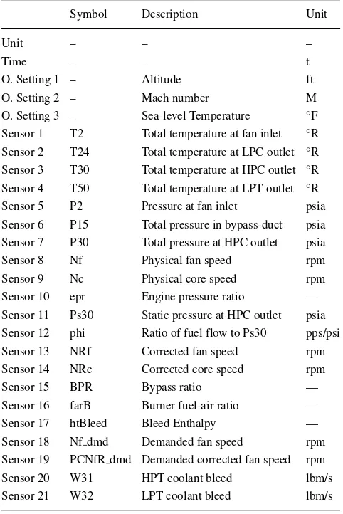
The raw values in the dataset are regarded as a snapshot of the parameters taken during a single cycle, and each column corresponds to a different variable (see Table2). The first two columns are respectively the trajectory unit

Table 1 Characterstics of PHM08 challenge dataset

Training Test Final test

Number of trajectories 218 218 435

Regimes 6 6 6

Fault modes One (high-pressure compressor degradation)

Maximum unit length 357 364 298 Minimum unit length 128 15 20

Table 2 PHM08 challenge dataset parameters available to participants

as sensor data [48]

Symbol Description Unit

Unit – – –

Time – – t

O. Setting 1 – Altitude ft

O. Setting 2 – Mach number M

O. Setting 3 – Sea-level Temperature ◦F Sensor 1 T2 Total temperature at fan inlet ◦R Sensor 2 T24 Total temperature at LPC outlet ◦R Sensor 3 T30 Total temperature at HPC outlet ◦R Sensor 4 T50 Total temperature at LPT outlet ◦R Sensor 5 P2 Pressure at fan inlet psia Sensor 6 P15 Total pressure in bypass-duct psia Sensor 7 P30 Total pressure at HPC outlet psia

Sensor 8 Nf Physical fan speed rpm

Sensor 9 Nc Physical core speed rpm

Sensor 10 epr Engine pressure ratio — Sensor 11 Ps30 Static pressure at HPC outlet psia Sensor 12 phi Ratio of fuel flow to Ps30 pps/psi Sensor 13 NRf Corrected fan speed rpm Sensor 14 NRc Corrected core speed rpm

Sensor 15 BPR Bypass ratio —

Sensor 16 farB Burner fuel-air ratio —

Sensor 17 htBleed Bleed Enthalpy —

Sensor 18 Nf dmd Demanded fan speed rpm Sensor 19 PCNfR dmd Demanded corrected fan speed rpm Sensor 20 W31 HPT coolant bleed lbm/s Sensor 21 W32 LPT coolant bleed lbm/s

LPC/HPClow/high-pressure compressor,LPT/HPTlow/high-pressure turbine

number and time of operational cycles, while columns 3, 4 and 5 are operational settings. The remaining are different sensor labels from operations.

4 Prognostic model

The contribution of this study is to provide a multiple-regime normalisation and health indicator (HI) assignment as an output to neural network function. PHM08 data exhibit multiple operational regimes that may cause prognostic models without a detailed pre-processing step to have a risk of excessive error rates. Main challenges encountered during the data pre-processing step include determining the initial wear level, filtering noise and calculating HI. The differences between the initial wear levels can occur due to service-life differences. Although they are not considered abnormal, they directly affect the analysis of useful operational life of the engines. Noise filtering is a non-trivial undertaking while assessing the true state of system’s health. The identification of operability margins for the HI is a crucial step to determine safe operation regions of engines.

Data pre-processing is performed to transform raw data into an understandable format that can be consumed by an automated filtering process. Data analysis that is based on poorly partitioned data could produce misleading outcomes. Therefore, proper pre-processing of data must be given consideration before carrying out the remaining useful life calculations.

Each trajectory in the dataset includes some noise, has a specific initial wear level and is scrambled by the effects of operational conditions. The algorithm is, thereby, required to deal with unfolding these complexities.

Figure2shows raw sensor signals of a specific training trajectory. The sensors represent various system conditions and performance measurements.

Figure3shows the behaviour of a single sensor (sensor 4—column 9). It can be seen in the plot that the data are highly scattered and it is hard to perform a regression that represents the system degradation. A meaningful observation from the raw sensor is, therefore, not possible without first carrying out a transform that allows better

0 50 100 150 200 250

Time, in Operational Cycles 0

500 1000 1500 2000 2500 8000 8500 9000 9500

Raw Sensor Readings

Fig. 2 Raw data characteristics

0 50 100 150 200 250

Time, in Operational Cycles 1000

1050 1100 1150 1200 1250 1300 1350 1400 1450

Total temperature at LPT outlet °R

Fig. 3 Sensor 4

identification of the degradation pattern within the noisy and scattered sensors.

In order to provide a HI that is useful for prognosis, a data processing approach is required that includes feature extraction, data cleaning and feature selection. The characteristic features of raw data and system conditions are extracted, and then outliers are removed.

The steps taken from new data intake to the neural network fitting and multistep ahead RUL calculations are shown in Fig.4. The following sections describe the steps in more detail.

4.1 Data pre-processing

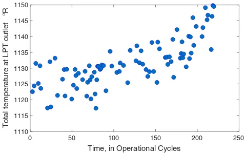
Based on data observations obtained from a single sensor such as on Fig.3, it can be noticed that certain sets of data points align in similar regions. When one looks only at data from a specific region (say those betweeny-values of 1110 to 1150 as seen on Fig.5), it becomes apparent that readings align in a domain (ϑri) as suggested in Eq.4. Raw sensor

Fig. 4 Flowchart representing data processing and multistep ahead

0 50 100 150 200 250

Time, in Operational Cycles

1110 1115 1120 1125 1130 1135 1140 1145 1150

Total temperature at LPT outlet °R

Fig. 5 Sensor 4 (yaxis limited)

values in this range could be regarded as coming from a certain operational regime.

4.1.1 Regime identification and clustering

The first step of data processing is to identify these oper-ational regimes in all trajectories. The number of regimes can be found by finding the number of clusters in the oper-ational settings. For the PHM08 challenge dataset, multiple regime clustering was carried out via various methods, such as k-means [65], Gaussian mixture models[66], nearest-neighbour clustering [67], Fuzzy c-means [68] and neural network clustering [69].

Further observations reveal that the three operational settings (altitude, mach number and sea-level temperature as given in Table 2) are concentrated in six different clusters, pointing out six operating regimes including many data points at each sensor parameter as such in Fig. 3. To identify the regimes in sensor parameters that are highly scattered due to the operational settings, a clustering analysis is needed to group data points in such a way that the operational setting variables in the same group are more similar (with regard to their maximum and minimum values) to each other than to those in other groups. Operating condition 3 has constant values that are correlated with different regimes (see Table 3). This paper utilises that correlation to assign the different operating regimes.

The mathematical expression for clustering is given by;

f (xp)=argk=1,...Rfind(x=k) (10)

where argk=1,...Rfind(x = k) defines the index of the

occurrence of regimes,k, in the data,x, andRdenotes the number of the unique values in operating condition 3.

An illustrative sample of the sensors after regime assignment is given in Fig.6. Comparing to Fig.5in which the plot’s axis is limited by a certain data range, all six regimes are grouped successfully, and if a correlation is carried out to cluster and standardise the data into a common regime, sensors can provide more meaningful information on system degradation.

4.1.2 Normalisation and re-assembling

A normalisation method can carry out adjustments by returning raw values into a common scale (for example the z-score). The z-score is a dimensionless quantity that is the result of subtracting the population mean of each regime from each individual raw sensor value and then dividing the difference by the population standard deviation.

Computing a z-score for each regime requires knowing the mean and standard deviation of the regime population of each sensor to which a data point belongs. The equation to calculate the standard score of a raw value is given as;

Nxr = x

r _−μr

σr ,∀r (11)

where, x is the raw data values for regime r, σ is the population standard deviation andμis the population mean or that feature. Since the data are made up of n scalar observations, the population standard deviation is:

σr =

n

i=1(xir−μ r i)2

n (12)

and the population mean is:

μr = 1 n

n

i=1

x_ir (13)

Table 3 Operating conditions

and regimes Regime Operating condition 1 Operating condition 2 Operating condition 3

Max Min Max Min Constant

1 42.008 41.998 0.842 0.840 40

2 35.008 34.998 0.842 0.840 60

3 25.008 24.998 0.622 0.620 80

4 10.008 9.998 0.252 0.250 20

5 20.008 19.998 0.702 0.700 0

Fig. 6 Clustered regimes for sensor 4

A key point in multiple regime normalisation is that calculatingzrequires each regime’s population mean and deviation over all entire time series. This will baseline the entire dataset at once.

This process is applied to all regimes and to all sensors separately, the standardised sensors are reassembled to form the normalised dataset. Figure 7 shows all standardised sensors in a training trajectory.

4.1.3 Sensor selection

Next, it is required to evaluate how well the sensors correlate with the degradation pattern. Signals which do not ade-quately correlate with a monotonic exponential trend will be removed [58]. To that end, the three prognostic parame-ter choosing measures of monotonicity, prognosability and trendability are used to identify the meaningful sensors [70].

Monotonicity is a straightforward measure to characterise the underlying positive or negative trend of the sensors. It is defined by:

Monotonicity=mean

#pos_dxd

n−1 − #neg_dxd

n−1

(14)

0 50 100 150 200 250

Time, in Operational Cycles -4

-2 0 2 4 6 8 10

Normalised Dimensions

Fig. 7 Normalised sensors

wherenis the number of training trajectories in a particular history. The monotonicity of a sensor population is calcu-lated by the average difference of the fraction of positive and negative derivatives for each path. A monotonicity measure outcome close to 1 indicates that the sensor is monotonic and useful for RUL estimation, whereas an outcome close to 0 indicates that the sensor is a non-monotonic signal and not suitable for further consideration.

Prognosability is calculated as the deviation of the failure points for each path divided by the average variation of the sensor during its entire lifetime. This measure is exponentially weighted to provide the desired 0 to 1 scale:

Prognosability=exp

− σfailure

μfailure−μhealthy

(15)

The prognosability measures close to 1 indicate that the failure thresholds are similar and the sensors are available for prognosis, whereas the measures close to 0 show that the failure points are different than each other and the sensors are incapable for the prognostic calculations.

Trendability is given by the minimum absolute correlation computed among all the training trajectories. The mathe-matical expression is represented by:

Trendability=mincorrcoeffij (16)

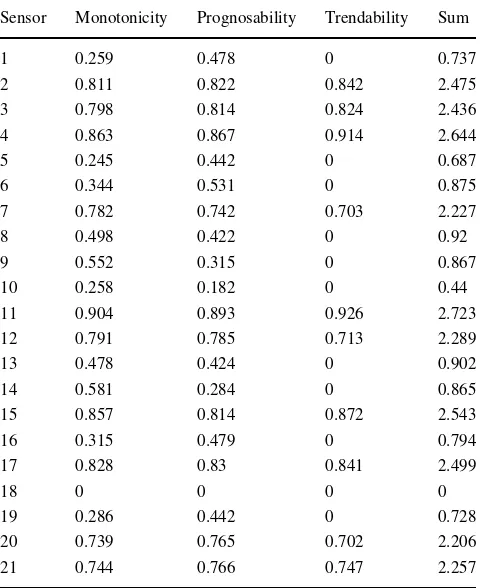
Results of trendability, monotonicity and prognosability parameter features are used to compare whether the candidate sensors are useful for individual-based prognosis. By quantifying these results for given results, the parameters can be used along with any traditional optimisation methods [70]. By defining a fitness function as a sum of these three-prognostic parameter choosing metrics, the sensors can be compared to determine the most suitable ones. It has been observed that the sensors can provide useful degradation information when each measurement is close to “1”. With respect to the results of prognostic parameter choosing measures in Table4, the ten sensors 2, 3, 4, 7, 11, 12, 15, 17, 20 and 21 are accepted as useful for the calculation of HI and applied in the following sections.

Figure 8 shows these normalised useful sensors to be used in further prognosis applications.

4.1.4 Health indicator assessment

To produce a single adjusted cycle (s), multiple readings from useful sensors (x) are aggregated by taking the mean of all sensors at each time step (i).

si=

1

n

n

j=1

xj i (17)

Table 4 Results of prognostic parameter suitability metrics

Sensor Monotonicity Prognosability Trendability Sum

1 0.259 0.478 0 0.737

2 0.811 0.822 0.842 2.475

3 0.798 0.814 0.824 2.436

4 0.863 0.867 0.914 2.644

5 0.245 0.442 0 0.687

6 0.344 0.531 0 0.875

7 0.782 0.742 0.703 2.227

8 0.498 0.422 0 0.92

9 0.552 0.315 0 0.867

10 0.258 0.182 0 0.44

11 0.904 0.893 0.926 2.723

12 0.791 0.785 0.713 2.289

13 0.478 0.424 0 0.902

14 0.581 0.284 0 0.865

15 0.857 0.814 0.872 2.543

16 0.315 0.479 0 0.794

17 0.828 0.83 0.841 2.499

18 0 0 0 0

19 0.286 0.442 0 0.728

20 0.739 0.765 0.702 2.206

21 0.744 0.766 0.747 2.257

there is a risk that neural network might learn the noise during the training stage. Therefore, a regression model is used to describe the relationship between the adjusted cycle index (s, the aggregated variable of Eq.17) and the HI. As shown in Fig.9, the adjusted cycle index represented by blue line includes noise and a fitted model represented by red line is used as the output term for the network training. Since the trained network function will be used with different raw training inputs and accordingly will estimate their HIs, the noise in the output of the network training should be

0 50 100 150 200 250

Time, in Operational Cycles -4

-3 -2 -1 0 1 2 3 4

Normalised Dimensions

Fig. 8 Useful normalised sensors

Fig. 9 Adjusted cycle and HI

carefully considered. A certain output for network training might produce biased results for alternative trajectories. However, if a fitted HI from the noisy-adjusted cycle is used in training, it will be possible to standardise the network estimations for each novel estimation.

To preserve the original degradation pattern, the follow-ing two-term power series fittfollow-ing model is used to identify a standard HI.

y= ˘asb˘+ ˘c+ε (18)

where an approximation to a power-law distribution sb˘

includes two fitting terms a˘ and c˘. The main reason for selection of this fitting approach is that the fitted HIs, y, for training trajectories have only increasing values and early stages are behaving in such a way that the fitting has minimum wear increase levels. Observing from the adjusted cycles that the failure occurs at a certain stage of operations and the system before this point is relatively stable, the two-term power series model can describe the hypothetical degradation model effectively. It is noticed that while the failure starts and ends at particular time points at each trajectory differs, the trajectories fail at similar wear levels. Since this research estimates the RULs by a similarity-based prediction method, the length of training trajectory time series after the most similar location is accepted as the RUL instead of identifying a threshold point and the HI’s crossover.

4.2 Neural network training

normalisation, all testing and training trajectories should be normalised at once in order to adjust initial wear and threshold points. To avoid these issues, a neural network fitting model is designed as an alternative method to map between raw training inputs and an HI output.

The network is a feed-forward model which takes a set of input vectors (raw data), and then arranges another set of output vectors (HI) as a target data. Neurons, which are the building blocks of the neural network, evaluate these input state variables. The nodes in the hidden layer are performed by the following function.

z=fx

b+

n

i₌1

wixi

(19)

where the state variables(xi)are multiplied by fixed

real-valued weights (wi) and bias b is added. The neuron’s

activation z is obtained as a result of the nodes and the nonlinear activation function of neuronsfx[71,72].

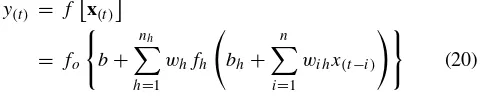
For the network structure shown in Fig.10, the general network equation can be denoted by

y(t) = f

x(t)

= fo

b+

nh

h=1

whfh

bh+ n

i=1

wihx(t−i)

(20)

The network used for fitting function is a two-layer feed-forward network, with a sigmoid transfer function(fh)in

the hidden layer and a linear transfer function in the output layer (fo). The default number of hidden neurons is not

set to a certain number. Instead, an outer loop is designed with an increasing number of hidden neurons. The optimum hidden layer size is accepted according to the mean squared difference between the initial output series and what is estimated.

The first step to train the network structure is the con-figuration of input and output series. Inputs are configured

Fig. 10 Neural network learning stage

as “10×time” cell of useful raw sensor data while the target series are configured as a 1×time cell of the HI calculated in the previous section. In order to increase the accuracy of configuration between trained outputs and targets, multi-ple networks are designed in a double-loop design over the increasing number of hidden nodes of an outer loop and ran-dom weight initialisations of an inner loop [73]. Both loops terminate when minimum desired error occurs and mean squared error is used to reduce error numbers in training. At the end of both loops, the least erroneous network is used to choose the best design mode for validation.

Neural networks with multiple nonlinear hidden layers are effective models that can contain a large number of parameters, but both overfitting and computational overhead might lead to poor network training, especially when data are presented to the predictions of numerous different large neural networks at testing stages [74]. These network training could memorise the samples for the specific training case, but there is always a risk that they cannot be trained properly to generalise the upcoming testing cases. That is why artificial neural networks (similar to other artificial intelligent machine learning models) are prone to overfitting the training data [75].

In order to avoid such training problems, this works applies Bayesian regularisation method into the network training [76, 77]. Other well-known alternatives to the Bayesian method are the “Levenberg-Marquardt” and “scaled conjugate gradient” algorithms [78]. When the Levenberg-Marquardt model is used to avoid overfitting, the network training needs more memory but less time and it automatically stops when generalisation concludes improving, as specified by an increase in the mean squared errors. In the case of the “scaled conjugate gradient”, the regularisation requires less memory and it is available when the training data is short. Bayesian regularisation requires more time in comparison to other methods due to the adaptive weight minimisation but can result in satisfactory generalisations from difficult or noisy datasets [79].

The training function in the Bayesian model is based on Gauss-Newton approximation to the Hessian matrix. It updates the weight and bias values according to Levenberg-Marquardt optimisation [76]. This function diminishes a compound of squared errors and weights in pursuance of reducing the computational overhead and overfitting in training, and then defines the correct compound so as to produce a convenient network generalisation [77]. Although this definition of Bayesian regularised neural network can take longer to train, it obtains a better solution compared to other methods.

similar pattern, but it is contaminated with noise as expected (Fig.11). In this case, the response is matching with the original HI used in network training, and the network can now be put to use on new inputs. The analysis of the network response is performed with a test trajectory (Fig.12). While the length and initial wear level are different, the model could accurately identify HI curve of the inserted data.

4.2.1 Network library

Although the network function trained with certain data provides desired results, there is always a risk that if the network is trained with other input and output values, the estimations might result in undesired estimations due to different weight and bias values. To that end, alternative neural networks, fN N, with inputs and outputs from

different trajectories are trained on similar problems and each trained function is stored in a network library,L.

L{i} = fN N_{i}, i=1,2,· · ·, nl (21)

L_{i} = yiN N, i=1,2,· · ·, nl (22)

wherenlis the number of trained functions in the library. When all novel trajectories have been inserted into that library, there will be multiple estimations for a single-input trajectory. Figure 13 demonstrates such a set of network library outputs that result in similar exponential growth patterns. The network library is formed of multiple network functions that have been trained by different data. When the same input data,x, is applied to these functions, they result in similar outputs,y₁N N_:nl, no matter which trajectory is used in their training.

Each trajectory in Fig.13is an estimated output of the same raw training input resulting from a trained network function in the library. The consistency between different estimations shows that ANN functions trained with different

Fig. 11 Neural network validation stage

Fig. 12 Neural network estimation stage

trajectories could adequately assign similar HI outputs which start at similar initial wear levels and end at similar threshold points.

Considering that the library results in multiple estima-tions for a single input, a final HI estimation similar to Section 4.1.4 is applied for dimensionality reduction. For further stages, referring to Eq.17, the moving average of all these alternative network results is applied to filter a final HI.

sr =

1

p

r+p

q=r

1

nl

nl

j=1

yj qN N (23)

where the random sequence sr is the mean of p-moving

average of nl number of HIs. As the window size of p -moving average is specified as a numeric duration scalar for next steps, the average contains the parameters in the current location plus upcoming neighbours. When the window is

expanded prior to thesr, the centred average equation can

be expressed as:

sr =

1 2p+1

r+p

q=r−p

1

nl

nl

j₌1

yN N_{j q} (24)

Directional window is a temporary duration matrix, and its size is formed of two distinct elements, the positive integer scalars of moving average windows size “p” and the number of library estimations “n”. This moving average helps to smooth out HI action by filtering out the “noise” from the network library results. However, the characteristic starting and failure points are of critical importance to the defining HI feature and they are required to be included in the filtered outputs. Regarding the prior and posterior values as well as the sequence itself, the exact windows size calculation is over(2p+1)×nelements.

When initial starting and the final ending points are concerned, the modified moving average method for a full matrix of library estimations is calculated by;

si=

⎧ ⎪ ⎪ ⎪ ⎪ ⎪ ⎪ ⎪ ⎪ ⎨ ⎪ ⎪ ⎪ ⎪ ⎪ ⎪ ⎪ ⎪ ⎩ 1

p+i

p+i q=1 1

n

n

j=1yj qN N ifi−p <0

1

p+(l−i+1)

p₊(l₋i₊1) q=i

1

n

n

j=1yj qN N ifi+p > l

1 2p+1

r+p q=r−p 1n

n

j=1yj qN N ifi−p >=0

and ifi+p <=l

(25)

wherelis the length of the estimations. Short dimensions to operate along the matrix are specified as a positive integer scalar for starting points and an integer scalar smaller than the length of matrix for the ending points. The rest have the full dimensions that moving average operates along the direction of the defined window slide. Thus, the moving average method could be applied to starting and ending points of the time series.

4.3 Similarity-based distance evaluation

Once different neural networks are trained to form a generalisation of the input-output relationship, the network library is used to estimate all HIs of training and test trajectories in the same dataset. The goal of supervised similarity learning is to learn from samples a similarity model that measures how similar or related two trajectories are. This method is closely related to distance metric learning in which the task of learning is a distance function over training and test trajectories. In practice, the similarity learning ignore the condition of identity of indiscernibles and learn the best fitting objects.

RUL estimation of test trajectories is used as a valid case to compare the test case against the full operational periods.

The difference between the two trajectories is computed as a similarity measure.

This similarity can be expressed as a distance between two vectors and is calculated as:

d(tr,te)=

n

i=1

(tei−tri)2. (26)

whereteis the test trajectory,tr is the corresponding part andnis the length of test trajectory.

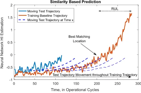
In Fig.14, pairwise distance between two sets of obser-vations is initially calculated at time step “1”. However, the best-matching training units can be in the later part of the curve. The testing curve is, therefore, moved step by step to the end of the base curve. The pairwise distance is cal-culated and stored for each step by the following equation;

d(te,tr)(j )=

ntr

j=nte nte

i=1

tei−tri+j

2

. (27)

wherentris the length of the base curve (training trajectory)

andnteis the length of test trajectory.

After the testing curve is moved to the end of a baseline case, the location of the best-matching units is calculated by identifying the minimum pairwise distance value.

Mn(te,tr)=min

d(te,tr)(1), d(te,tr)(2),· · ·, d(te,tr)ntr−nte

(28)

The location of the best-matching part at the training baseline,Lcte,tr, is calculated by:

Lct e,t r = arg find

d(te,tr)(j )=Mn(te,tr) ; (29)

j = 1,2,· · ·(ntr−nt e) (30)

The prior parts before this location are removed and the followings are used for further estimation as seen on Fig.15.

Fig. 15 Top similarities and RUL calculation

4.3.1 RUL estimation

The identification of the best-matching location and minimum Euclidean distance is used for the calculation of RUL for each baseline (training trajectory).

RULt e,t r =nt r−(nt e+Lct e,t r) (31)

The length of time series after the calculated location of the best-matching part, Lt e,t r, equals to the remaining

useful life of the test trajectory. As a single calculation with a single baseline can be expanded to all training trajectories, the calculations with more training data samples could increase prediction accuracy in multistep ahead estimations. The final RUL is estimated by the mean value of corresponding RUL calculations of the minimum ten distance values of all baselines. A demonstration of these best-matching trajectory parts is shown in Fig.15.

5 Results

There have been several thousand downloads of C-MAPSS dataset files since their first release in 2008, and as of 2014, more than 70 papers referring to these datasets were found in the published literature [59].

The presented algorithm was applied to all trajectories in PHM08 data challenge and RUL was calculated for each test subset. The results were evaluated by the prognostic metrics shown in Table5. Several metrics are used here to allow for comparison of findings on several different levels.

Table 5 Prognostic metrics

Metric Formula

Mean absolute error [80] MAE= 1

n

n

i=1

|ei| =

1

n

n

i=1

yi− ˆyi e=error

y=true RUL

ˆ

y=predicted RUL

n=number of predictions

Mean absolute percentage error [81,82] MAPE= 100

n

n

i=1

yi− ˆyi

yi

Mean square error [80] MSE= 1

n

n

i=1

ei2=

1

n

n

i=1

yi− ˆyi 2

False positive rate [83] F P (i)=

1 error > tF P

0 otherwise tF P, tF N=acceptable early/late prediction limits

False negative rate [83] F N (i)=

1 −error > tF N

0 otherwise

Anomaly correlation coefficient [82,83] ACC=

(π(i|j )−z#(i)) (z∗(i)−z#(i))

(π(i|j )−z#(i))2(z∗(i)−z#(i))2

z∗(i)=prediction variable

z#(i)=corresponding

history data value

Sample standard deviation [80,82] s=

1

n−1

n

i=1

(yi−μe)2 μe=sample mean of error

Mean absolute deviation from sample median [82] MADi=

1

n

n

i=1

|ei−M| M=median(e)median

Table 6 Performance of the developed model

Rank Scoring function MSE FPR (%) FNR (%) MAPE (%) MAE Corr. score Std. dev. MAD MdAD

1 5530.12 515.35 48.51 50.80 20.68 15.93 0.92 1.07 16.63 10.20

These metrics aim principally at performance validations for prognostics applications. Since they are mostly focused on applications where run-to-failure data are available, their usage has a particular importance for the model development stage where metric feedback could be used to integrate the prognostic procedures.

Table 7 shows the comprehensive set of metrics as computed from PHM08 Challenge leader board of final test set [59]. Ranking is established based on PHM scoring function, which is a weighted sum of RUL errors [82,83]. The following equations describe the scoring function.

Sc= ⎧ ⎪ ⎪ ⎨ ⎪ ⎪ ⎩

npr

i=1exp −e

a1

for e <0

npr

i=1exp

e

a₂

for e≥0

(32)

where “Sc” is the computed score, npr is the number of

predicted units andeis the error term. The scoring function is an asymmetric metric that penalises late predictions more than the early predictions, a1 = 13 and a2 = 10, due to the fact that late predictions imply more costly failure consequences. There is no upper penalty limit for predictions, and thereby, a single high error rate among the predictions in the dataset can dominate the final score. It is particularly risky for test units with a short history in which both early and late predictions are highly possible. In order to avoid such a risk, the maximum threshold value for RUL predictions is capped at 135. This value was gleaned from the training data (i.e. none exceeds 135)

and assumes that future unseen trajectories will adhere to that same characteristic. Also, it is observed that the trajectories shorter than 50-time cycles are prone to result in excessive early or late predictions. Considering the asymmetric characteristic of the scoring function, the range of the short trajectory RUL predictions is directly adjusted between 100 and 130.

The algorithm explained in this paper is applied to the validation dataset which contains 435 test samples and the results were sent to PCoE for performance validation. The model achieved a total score of 5530.12, which is the overall leading score at this time (see Tables6and7).

The distinguishing difference between false positive (FP) and false negative (FN) rates deserves a special consideration for final test validation. Their percentage can be compiled to measure the consistency and reliability of developed models. As seen in Table7, the positive rates in the leader board are predominantly higher than the negative rates. This might be a direct result of a biased merging of multiple RUL estimates through a weighted calculation due to the high penalty scores for late predictions. However, the early predictions might also dominate the final score in a real case scenario and might result in catastrophic failures. This work did not apply any weighting method between early and late predictions. Accordingly, the calculated rates are very close to each other, and the developed model could be regarded consistent and reliable in terms of FP and FN rates when comparing the results in Table7.

Table 7 Leader board of PHM08 final dataset (published works) [59]

Rank Scoring function MSE FPR (%) FNR (%) MAPE (%) MAE Corr. score Std. dev. MAD MdAD

1 5636.06 546.60 64.83 31.72 19.99 16.23 0.93 1.01 16.33 11.00

2 6691.86 560.12 63.68 36.32 17.92 15.38 0.94 1.03 16.29 8.08

3 8637.57 672.17 61.38 23.45 20.72 17.69 0.92 1.09 17.79 11.00

4 9530.35 741.20 58.39 39.54 34.93 20.19 0.90 1.22 20.17 15.00

5 10571.58 764.82 58.85 41.15 32.60 20.05 0.91 1.22 20.41 14.23

6 11572∗ – – – – – – – – –

7 14275.60 716.65 59.77 37.01 21.61 18.16 0.90 1.17 18.57 11.00

8 19148.88 822.06 56.09 41.84 30.25 20.23 0.88 1.29 20.89 13.00

9 20471.33 1000.06 51.95 48.05 33.63 22.44 0.88 1.42 24.05 14.78

10 22755.85 1078.19 62.53 35.40 39.90 24.51 0.86 1.45 24.08 20.00

11 25921.26 854.57 34.25 64.83 51.38 22.66 0.86 1.36 21.49 16.00

6 Conclusion and future work

The algorithm developed in this work has been effective for RUL calculations of C-MAPPS datasets. A data-driven filtering approach can successfully assign HI targets for similarity-based remaining useful life calculation. Since the multiple regime normalisation is applied by the trained neural network, there is no need for the standardisation of the entire dataset at once. Thereby, both training and test trajectories could be processed individually by considering their initial wear levels.

During the course of model development, it was observed that a mathematically defined synthetic output vector also performed satisfactorily for neural network training. Due to the constraints of the scoring metrics (one-time limited submission and variance in initial wear levels), this work used a step by step HI (output) data processing.

A smart selection system produced a library of synthetic output models and the best-matching degradation model was selected for the raw test data. For future works, we envision to explore for the developed network model with automated output selection and normalisation for various failure mode situations.

Funding information The material is based upon work supported in

part by NASA under award NNX12AK33A with the Universities Space Research Association

Open Access This article is distributed under the terms of the

Creative Commons Attribution 4.0 International License (http:// creativecommons.org/licenses/by/4.0/), which permits unrestricted use, distribution, and reproduction in any medium, provided you give appropriate credit to the original author(s) and the source, provide a link to the Creative Commons license, and indicate if changes were made.

Publisher’s Note Springer Nature remains neutral with regard to

jurisdictional claims in published maps and institutional affiliations.

References

1. Goebel K, Saha B, Saxena A (2008) A comparison of three data-driven techniques for prognostics. In: 62nd Meeting of the society for machinery failure prevention technology (mfpt), pp 119–131 2. Randall RB (2011) Vibration-based condition monitoring:

indus-trial, aerospace and automotive applications. Wiley

3. Schwabacher M, Goebel K (2007) A survey of artificial intelligence for prognostics. In: Aaai fall symposium, pp 107–114 4. Brown D, Kalgren P, Roemer M (2007) Electronic prognostics-a cprognostics-ase study using switched-mode power supplies (smps). IEEE Instrum Measur Mag 10(4):20–26

5. Bektas O, Alfudail A, Jones JA (2017) Reducing dimensionality of multi-regime data for failure prognostics. J Fail Anal Prev 17(6):1268

6. Si XS, Wang W, Hu CH, Chen MY, Zhou DH (2013) A wiener-process-based degradation model with a recursive filter algorithm for remaining useful life estimation. Mech Syst Signal Process 35(1):219–237

7. Chinnam RB, Mohan P (2002) Online reliability estimation of physical systems using neural networks and wavelets. Int J Smart Eng Sys Des 4(4):253–264

8. Sheldon J, Lee H, Watson M, Byington C, Carney E (2007) Detection of incipient bearing faults in a gas turbine engine using integrated signal processing techniques. In: Annual forum proceedings-American helicopter society, vol 63. American Helicopter Society, Inc, p 925

9. Camci F (2005) Process monitoring, diagnostics and prognostics using support vector machines and hidden Markov models. Ph.D. thesis. Wayne State University, Detroit

10. Liu Q, Dong M, Peng Y (2012) A novel method for online health prognosis of equipment based on hidden semi-Markov model using sequential monte carlo methods. Mech Syst Signal Process 32:331–348

11. Byington CS, Watson M, Edwards D (2004) Data-driven neural network methodology to remaining life predictions for aircraft actuator components. In: Aerospace conference, 2004. Proceedings. 2004 IEEE, vol 6. IEEE, pp 3581–3589

12. Byington CS, Watson M, Edwards D (2004) Dynamic signal analysis and neural network modeling for life prediction of flight control actuators. In: Proceedings of the American helicopter society 60th annual forum

13. Saha B, Poll S, Goebel K, Christophersen J (2007) An integrated approach to battery health monitoring using bayesian regression and state estimation. In: Autotestcon, 2007 IEEE. IEEE, pp 646– 653

14. Pola DA, Navarrete HF, Orchard ME, Rabi´e RS, Cerda MA, Olivares BE, Silva JF, Espinoza PA, P´erez A (2015) Particle-filtering-based discharge time prognosis for lithium-ion batteries with a statistical characterization of use profiles. IEEE Trans Reliab 64(2):710–720

15. Hong S, Zhou Z (2012) Application of gaussian process regression for bearing degradation assessment. In: 2012 6th International conference on new trends in information science and service science and data mining (ISSDM). IEEE, pp 644–648

16. Chiach´ıo J, Chiach´ıo M, Sankararaman S, Saxena A, Goebel K (2015) Condition-based prediction of time-dependent reliability in composites. Reliab Eng Syst Safety 142:134–147

17. Medjaher K, Zerhouni N (2013) Hybrid prognostic method applied to mechatronic systems. Int J Adv Manuf Technol 69(1-4):823–834

18. Perez A, Moreno R, Moreira R, Orchard M, Strbac G (2016) Effect of battery degradation on multi-service portfolios of energy storage. IEEE Trans Sustain Energy 7(4):1718–1729

19. P´erez A, Quintero V, Rozas H, Jaramillo F, Moreno R, Orchard M (2017) Modelling the degradation process of lithium-ion batteries when operating at erratic state-of-charge swing ranges. In: International conference on control, decision and information technologies

20. P´erez A, Quintero V, Rozas H, Jimenez D, Jaramillo F, Orchard M (2017) Lithium-ion battery pack arrays for lifespan enhancement. In: 2017 CHILEAN Conference on electrical, electronics engi-neering, information and communication technologies (CHILE-CON). IEEE, pp 1–5

21. Jouin M, Gouriveau R, Hissel D, P´era MC, Zerhouni N (2016) Degradations analysis and aging modeling for health assessment and prognostics of pemfc. Reliab Eng Syst Safety 148:78–95 22. Pastor-Fern´andez C, Widanage WD, Chouchelamane G, Marco

J (2016) A soh diagnosis and prognosis method to identify and quantify degradation modes in li-ion batteries using the ic/dv technique. In: IET Conference publications (CP691), pp 1–6 23. Saha B, Celaya JR, Wysocki PF, Goebel KF (2009) Towards

24. Wang T (2010) Trajectory similarity based prediction for remaining useful life estimation. University of Cincinnati 25. Zaidan MA, Mills AR, Harrison RF (2013) Bayesian framework

for aerospace gas turbine engine prognostics. In: Aerospace conference, 2013 IEEE. IEEE, pp 1–8

26. Sikorska J, Hodkiewicz M, Ma L (2011) Prognostic modelling options for remaining useful life estimation by industry. Mech Syst Signal Process 25(5):1803–1836

27. Kothamasu R, Huang SH, VerDuin WH (2006) System health monitoring and prognostics—a review of current paradigms and practices. Int J Adv Manuf Technol 28(9–10):1012–1024 28. Peng Y, Dong M, Zuo MJ (2010) Current status of machine

prog-nostics in condition-based maintenance: a review. International Journal of Advanced Manufacturing Technology 50(1–4):297– 313

29. Niknam SA, Kobza J, Hines JW (2017) Techniques of trend analysis in degradation-based prognostics. Int J Adv Manuf Technol 88(9–12):2429–2441

30. Xiao Q, Fang Y, Liu Q, Zhou S (2018) Online machine health prognostics based on modified duration-dependent hidden semi-Markov model and high-order particle filtering. Int J Adv Manuf Technol 94(1-4):1283–1297

31. Zhou Y, Xue W (2018) Review of tool condition monitoring methods in milling processes. Int J Adv Manuf Technol, 1–15 32. Heimes FO (2008) Recurrent neural networks for remaining useful

life estimation. In: International Conference on prognostics and health management, 2008. PHM 2008. IEEE, pp 1–6

33. Mahamad AK, Saon S, Hiyama T (2010) Predicting remaining useful life of rotating machinery based artificial neural network. Comput Math Appl 60(4):1078–1087

34. Tian Z (2012) An artificial neural network method for remaining useful life prediction of equipment subject to condition monitor-ing. J Intell Manuf 23(2):227–237

35. Bonissone PP, Goebel K (2001) Soft computing applications in equipment maintenance and service. In: IFSA World Congress and 20th NAFIPS international conference, 2001. Joint 9th. IEEE, pp 2752–2757

36. Yan J, Liu Y, Han S, Qiu M (2013) Wind power grouping forecasts and its uncertainty analysis using optimized relevance vector machine. Renew Sustain Energy Rev 27:613–621

37. Benkedjouh T, Medjaher K, Zerhouni N, Rechak S (2015) Health assessment and life prediction of cutting tools based on support vector regression. J Intell Manuf 26(2):213–223

38. Widodo A, Yang BS (2011) Machine health prognostics using survival probability and support vector machine. Expert Syst Appl 38(7):8430–8437

39. Saxena A, Wu B, Vachtsevanos G (2005) Integrated diagnosis and prognosis architecture for fleet vehicles using dynamic case-based reasoning. In: Autotestcon, 2005. IEEE, pp 96–102

40. Byington CS, Watson M, Edwards D, Dunkin B (2003) In-line health monitoring system for hydraulic pumps and motors. In: Aerospace conference, 2003. Proceedings. 2003 IEEE, vol 7. IEEE, pp 3279–3287

41. Watson M, Byington C, Edwards D, Amin S (2005) Dynamic modeling and wear-based remaining useful life prediction of high power clutch systems©. Tribol Lubric Technol 61(12):38 42. Saha B, Goebel K, Poll S, Christophersen J (2009) Prognostics

methods for battery health monitoring using a Bayesian frame-work. IEEE Trans Instrum Measur 58(2):291–296

43. Gebraeel N (2006) Sensory-updated residual life distributions for components with exponential degradation patterns. IEEE Trans Autom Sci Eng 3(4):382–393

44. Amin S, Byington C, Watson M (2005) Fuzzy inference and fusion for health state diagnosis of hydraulic pumps and motors.

In: Annual Meeting of the North American fuzzy information processing society, 2005. NAFIPS 2005. IEEE, pp 13–18 45. Volponi A (2005) Data fusion for enhanced aircraft engine

prognostics and health management. Citeseer

46. Bar-Yam Y (2003) Complexity of military conflict: multiscale complex systems analysis of littoral warfare. Report to Chief of Naval Operations Strategic Studies Group

47. G¨unel A, Meshram A, Bley T, Schuetze A, Klusch M (2013) Statistical and semantic multisensor data evaluation for fluid condition monitoring in wind turbines. In: Proc. 16th Intl. conf. on sensors and measurement technology. Germany

48. Saxena A, Goebel K, Simon D, Eklund N (2008) Damage prop-agation modeling for aircraft engine run-to-failure simulation. In: International conference on prognostics and health management, 2008. PHM 2008. IEEE, pp 1–9

49. Uckun S, Goebel K, Lucas PJ (2008) Standardizing research meth-ods for prognostics. In: International conference on prognostics and health management, 2008. PHM 2008. IEEE, pp 1–10 50. Cempel C (2009) Generalized singular value decomposition in

multidimensional condition monitoring of machines—a proposal of comparative diagnostics. Mech Syst Signal Process 23(3):701– 711

51. Peel L (2008) Data driven prognostics using a Kalman filter ensemble of neural network models. In: International Conference on prognostics and health management, 2008. PHM 2008. IEEE, pp 1–6

52. Tumer IY, Huff EM (2003) Analysis of triaxial vibration data for health monitoring of helicopter gearboxes. J Vibr Acoust 125(1):120–128

53. Suo H, Wan J, Zou C, Liu J (2012) Security in the internet of things a review. In: 2012 international conference on computer science and electronics engineering (ICCSEE), vol 3. IEEE, pp 648–651 54. Kan MS, Tan AC, Mathew J (2015) A review on prognostic

techniques for non-stationary and non-linear rotating systems. Mech Syst Signal Process 62:1–20

55. Saxena A, Goebel K (2008) Phm08 challenge data set. NASA Ames Prognostics Data Repository (http://ti.arc.nasa.gov/project/ prognostic-data-repository), NASA Ames Research Center. Mof-fett Field

56. Boussif A (2016) Contributions to model-based diagnosis of discrete-event systems. Ph.D. thesis Universit´e de Lille1-Sciences et Technologies

57. Vassiliadis P (1998) Modeling multidimensional databases, cubes and cube operations. In: Tenth International conference on scientific and statistical database management, 1998. Proceedings. IEEE, pp 53–62

58. Wang T, Yu J, Siegel D, Lee J (2008) A similarity-based prognostics approach for remaining useful life estimation of engineered systems. In: International conference on prognostics and health management, 2008. PHM 2008. IEEE, pp 1–6 59. Ramasso E, Saxena A (2014) Performance benchmarking and

analysis of prognostic methods for cmapss datasets. Int J Prognostics Health Manag 5(2):1–15

60. Arbib MA (2003) The handbook of brain theory and neural networks. MIT Press

61. Murata N, Yoshizawa S, Amari Si (1994) Network information criterion-determining the number of hidden units for an artificial neural network model. IEEE Trans Neural Netw 5(6):865–872 62. Sim˜oes JM, Gomes CF, Yasin MM (2011) A literature review of

64. Frederick D, DeCastro J, Litt J (2007) User’s guide for the commercial modular aero-propulsion system simulation (c-mapss) (tech. rep.). Cleveland, p 44135

65. Lam J, Sankararaman S, Stewart B (2014) Enhanced trajectory based similarity prediction with uncertainty quantification. PHM 2014

66. McLachlan G, Peel D (2004) Finite mixture models. Wiley 67. Ramasso E (2014) Investigating computational geometry for

failure prognostics. Int J Prognostics Health Manag 5(1): 005

68. Sugeno M, Yasukawa T (1993) A fuzzy-logic-based approach to qualitative modeling. IEEE Trans Fuzzy Syst 1(1):7–31

69. Ultsch A (1993) Self-organizing neural networks for visualisation and classification. In: Information and classification. Springer, pp 307–313

70. Coble JB (2010) Merging data sources to predict remaining useful life–an automated method to identify prognostic parameters. University of Tennessee

71. Barad SG, Ramaiah P, Giridhar R, Krishnaiah G (2012) Neural network approach for a combined performance and mechanical health monitoring of a gas turbine engine. Mech Syst Signal Process 27:729–742

72. Krenker A, Kos A, Beˇster J (2011) Introduction to the artificial neural networks. INTECH Open Access Publisher

73. Heath G (2012) Declare net of neural network in mat-lab. [Online forum comment, Last Accessed 30 Nov 2017] https://www.mathworks.com/matlabcentral/profile/authors/29299 37-greg-heath

74. Srivastava N, Hinton GE, Krizhevsky A, Sutskever I, Salakhutdi-nov R (2014) Dropout: a simple way to prevent neural networks from overfitting. J Mach Learn Res 15(1):1929–1958

75. Lawrence S, Giles CL, Tsoi AC (1997) Lessons in neural network training: overfitting may be harder than expected. In: AAAI/IAAI. Citeseer, pp 540–545

76. MacKay DJ (1992) A practical Bayesian framework for backprop-agation networks. Neural computation 4(3):448–472

77. Foresee FD, Hagan MT (1997) Gauss-newton approximation to Bayesian learning. In: International conference on neural networks, 1997, vol 3. IEEE, pp 1930–1935

78. Demuth H, Beale M, Hagan M (2015) Matlab: neural network toolbox: user’s guide matlab r2015b. The MathWorks 2009 79. Demuth H, Beale M, Hagan M (2008) Neural network toolbox™

6. User’s guide, 37–55

80. Hyndman RJ, Koehler AB (2006) Another look at measures of forecast accuracy. Int J Forecast 22(4):679–688

81. Makridakis S, Andersen A, Carbone R, Fildes R, Hibon M, Lewandowski R, Newton J, Parzen E, Winkler R (1982) The accu-racy of extrapolation (time series) methods: results of a forecasting competition. J Forecast 1(2):111–153

82. Saxena A, Celaya J, Balaban E, Goebel K, Saha B, Saha S, Schwabacher M (2008) Metrics for evaluating performance of prognostic techniques. In: International conference on prognostics and health management, 2008. phm 2008. IEEE, pp 1–17 83. Goebel K, Saxena A, Saha S, Saha B, Celaya J (2011) Machine