Estimating 3D Scene Flow from Multiple 2D Optical Flows

Estimating 3D Scene Flow from Multiple 2D Optical Flows

Jonathan Ruttle

Michael Manzke

Rozenn Dahyot

ruttlejl@cs.tcd.ie

Michael.Manzke@cs.tcd.ie

Rozenn.Dahyot@cs.tcd.ie

Trinity College Dublin

School of Computer Science and Statistics

Graphics Vision and Visualisation Group

Abstract

Scene flow is the motion of the surface points in the 3D world. For a camera, it is seen as a 2D optical flow in the image plane. Knowing the scene flow can be very useful as it gives an idea of the surface geometry of the objects in the scene and how those objects are moving. Four methods for calculating the scene flow given multiple optical flows have been explored and detailed in this paper along with the ba-sic mathematics surrounding multi-view geometry. It was found that given multiple optical flows it is possible to es-timate the scene flow to different levels of detail depending on the level of prior information present.

1

Introduction

Optical flow is the 2D projection of the 3D scene flow onto the image plane. Optical flow has been around for nearly the last three decades [7], [6] and in that time the methods and techniques for calculate optical flow has im-proved greatly [4], [1]. It has been shown that it is possible to back-project the optical flow to compute the scene flow [11].

Knowledge of scene flow can help with a number of ap-plications including human motion capture [8] and can also help in determining the structure of the scene [12]. Combin-ing multiple optical flows in a sCombin-ingle scene flow could possi-ble detect and correct error in individual optical flows, this corrected optical flow could then be used for better video compression.

Traditionally calculating scene flow is done by matching pixels across two views of the same scene. This allows the depth information to be calculated and the two optical flows to be combined to generate the scene flow.

Vedula et al. presents three different scenarios for calcu-late scene flow [11]. The first scenario occurs when there

is complete knowledge of the surface of the object in the scene. In this case, Vedula shows that it is possible to calcu-late scene flow from a single camera. The second scenario occurs when there is knowledge of corresponding informa-tion between two image views and in this case it is possible to determine the scene flow from these two views. The third scenario is when there is no knowledge of the scene. In this situation, Vedula shows that, by using 51 cameras, possible scene flows can be generated and the results can be thresh-olded to reveal the moving objects in the scene.

Tian and Shah present a method for modelling the trans-lational and rotational motion of the objects in the scene and the scene flow is estimated by using a 5D histogram [9]. Torr et al. calculate matching feature points in each im-age to calculate the scene flow for the matched points and the scene structure [10].

2

Notation

All calculations assume knowledge of all extrinsic and intrinsic camera parameters. This includes the camera pro-jection matrixPiand the camera centrecifor each camera

i.

Pi=





p11 p12 p13 p14

p21 p22 p23 p24

p31 p32 p33 p34 

 (1)

ci=

    xc yc zc 1     (2)

Homogeneous coordinates are used for all 2D pixelsut i

in the image plane of cameraiat timetand all 3D points

xt_{in world space at timet.}

ut_i=   u v 1   (3)

xt=     x y z 1     (4)

Optical flowu˙t

i is the movement of a pixel over a time

interval from some previous time t0 to the current timet

where the interval|t−t0|is assumed to be of short duration.

˙ ut_i= u

t i−ut

0

i

t−t0 =   ˙ u ˙ v 0   (5)

Similarly the scene flowx˙tis:

˙ xt=x

t_−xt0

t−t0 =     ˙ x ˙ y ˙ z 0     (6)

The time is usually the frame index in the video stream and the optical flow is computed with successive framest−t0= 1.

2.1

Determining a 2D Pixel given a 3D

Point

A 3D pointxt in world space can be projected onto a 2D pixelut

i in the image plane by multiplication with the

projection matrixPi.

ut_i= Pixt (7)

Figure 1. In camera 1, a pixel ut

1 and a

cam-era centre c1 are used to calculate a 3D ray

of all possible pointsxt

1,uin the 3D world that

project onto pixelut

1.

2.2

Determining a 3D Ray given a 2D

Pixel

Given a single 2D pixelut

i, it is not possible to calculate

a single 3D pointxt

i,uwithout depth informationλti. It is

possible to calculate a 3D ray of points where any point on the ray will be projected onto the given 2D pixel ut

i.

Multiplying the pseudo-inverse of the projection matrixP+_i

(defined byP+_{= P}> _PP>−1_{) by the homogenous pixel} coordinate will results in some pointxt

i,uon the ray in the

scene in front of the camera.

xi,u= P+i ui (8)

Therefore a ray starting at the camera centreciand

con-tinuing on through this new pointxi,udescribes all

possi-ble points that could be projected onto the pixelut

i. A more

convenient way to describe this ray is Equation 10, where

~ nt

i,uis the unit vector fromcitoxi,uandλis some positive

number which represents the distance between the camera centre and the point that is being searched for. As seen in Figure 1.

~

nt_i,u= xi,u−ci

kxi,u−cik

(9)

xt_i,u=ci+λti~n t

i,u (10)

2.3

Determining a 3D Point given two

cor-responding Pixels

When two cameras are used and a pixel in each image

ut

iandutjare the projection of the same pointxt, it is

pos-sible to calculate the 3D position of that point. The points position will be the intersection of the two raysRt

i,u and

Rt

j,uformed by the pixels as described in section 2.2.

Figure 2. Two pixels ut

i and utj used to cal-culate pointxt_{by intersection the 2 raysR}t

i,u

and Rt

j,u. Where camera i = 1 and camera

j= 2.

and floating-point arithmetic it is quite unlikely that the rays will actually intersect, but they will pass close to each other. Therefore the midpoint of the two closest points ˆxt_i,uand

ˆ xt

j,uon the two rays can be used to give an approximate

solutionxt_{. If the distance between the two closest points}

ˆ xt

i,uandxˆtj,uis very large for example larger then the size

of a pixel then this may indicate that the two pixels do not refer to the same point and there may be error in the pixel matching.

2.4

Determining a 3D Scene Flow given

two corresponding Optical Flows

Similar to the situation in section 2.3 two 2D pixelsut i

andut_j with optical flows u˙t_i andu˙t_j both visualising the same 3D point and scene flow can be used to calculate the position of that pointxtand the direction and magnitude of that scene flowx˙t. As shown in Figure 3 the pixels can be converted into raysRt

i,uandRtj,uand the midpoint of the

two closest points reveal the position of the 3D pointxt_.

The optical flow can be used to calculate the last position of each of the pixels in the previous frameut0

i andut

0

j, by

subtracting the optical flow from the current position. These new pixels can be converted into raysRt0

i,uandRt

0

j,uand the

previous 3D pointxt0 can be calculated in the same way as in section 2.3. The vector from this previous pointxt0to the current pointxtis the scene flowx˙t.

2.5

Determining a range of possible points

and scene flows from a single pixel

Given a single pixelut

iwith optical flowu˙tiit is possible

to calculate a range of possible pointsxt_{and scene flowsx˙}t

which would project onto that pixel and optical flow. Using

Figure 3. Two optical flows used to calculate the scene flow of a point using two sets of intersection rays. Where camera i = 1 and cameraj= 2.

Figure 4. A range of possible scene flowsx˙t

given one optical flow u˙t_i after picking one possible pointxt. Where camerai= 1.

the optical flow it is possible to calculate the position of the pixel in the previous frameut_i0 =ut_i−u˙t_i. The 3D raysRt_i,u

andRt0

i,ucan be calculated for both the current and previous

pixel using the technique described in section 2.2.

The two rays can be seen in Figure 4, basically any vec-tor that connectsRt0

i,utoRti,uis a possible scene flow. The

Equation 10 gives you a range of possible points xt ₌

ci+λti~ni,tuby exploring all validλti. For each pointxton

Rt

i,u a range of possible previous pointsxt

0

can be found the same way onRt0

i,u. The time between frames will be

very small therefore it is possible to use this prior knowl-edge to place a maximum magnitude on the scene flow. It is possible to calculate the closest pointxˆt_i,0_uon the previous rayRt0

i,uto the currently selected pointxtonRti,u. Then

possible previous pointsxt0 =xˆt_i,0_u+λt_i0 ~nt_i,0_uby varying

λt0

i between plus and minus the maximum magnitude of the

3

Calculating 3D Scene Flow

Previously to calculate scene flow required knowledge of corresponding pixels, this in general requires pixels match-ing. The following four algorithms try to avoid this costly approach and use alternative methods by either finding sur-face points which can be projected into the cameras to find corresponding pixels or by overlapping all possible scene flows to find areas of concurrence.

3.1

Background Subtraction

Background subtraction is performed on each of the im-ages to determine which pixels belong to foreground ob-jects and which pixels belong to the background. A dense selection of equally distributed points is generated in the 3D world to be explored. Each point is projected into each of the cameras using Equation 7. If all the pixels relating to a point belong to a foreground object then the point is kept, otherwise the point is discarded. The remaining points form the solid shape of the object in the scene. The more cam-eras and the more points used the better the shape will be in approximating the object, but the more computationally expensive it will be.

To extract the surface points or visual hull, the remain-ing points are examined and inside points are discarded and surface points are kept. This is done by stepping through all the points and each time a border is crossed the point is kept otherwise it is discarded. At this point it is also noted which relative side of the object the point is on, this allows the relative cameras to be selected in determining the scene flow. The remaining points can be projected into the appro-priate cameras using the method described in section 2.1 and then the method described in section 2.3 can be used to determine the scene flow at that point.

3.2

Thresholding Optical Flow

Assuming that the only thing moving in the scene is the object then the background subtraction can be approx-imated by thresholding the optical flow results. The same method described in section 3.1 can be used but thresholded optical flow is used instead of the background subtraction results. This solution suffers from problems when the scene flow is in-line with one of the cameras. When this is the case then very little optical flow is seen in that camera and so it falls below the threshold, and therefore disappear in the final estimation of the scene flow.

3.3

Thresholding Scene Flow

This time the scene flow is calculated for all the points in the scene. The magnitude of each scene flow is measure and the ones below a threshold are discarded.

3.4

Histogram Data

A 6D histogram is created with the first three dimension as world position x y z, and the last three dimensions as scene flow components x˙ y˙, z˙. For every pixel in every camera the method described in section 2.4 is used to gen-erate possible scene flows, for every scene flow explored and relevant entry in the histogram is incremented.

The histogram is reduced to a 3D histogram by taking the maximum scene flow for each point, this is because no sin-gle point can have more than one scene flow. This new his-togram is then thresholded reducing the points to the ones with the highest values, these should be the surface points of the object as that is where the maximum concurrence should be.

4

Results

All four methods where implemented on the Human Eva II dataset [3]. Black et al. [2] optical flow algorithm was used to generate the optical flow for each of the four cam-eras. The two frames for the four cameras can be seen in Figure 5, this includes the result of a background subtrac-tion and the thresholded optical flow. The results of the four methods can be seen in Figure 6.

4.1

Background Subtraction

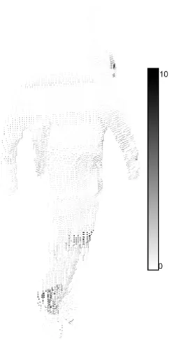
The scene flow derived using background subtraction is shown in Figure 6 (a). This can be visually inspected and it appears to be very accurate to when compared with the two frames of the scene. This method does require a framework which calculates the background subtraction. While a lot of human motion tracking algorithms use some form of back-ground subtraction it is not always possible to have a robust background subtraction. So while the result is very good it has its limitations in terms of the required prior knowledge of the background of the scene. Figure 7 shows the differ-ence between the original optical flow and the projection of the new scene flow in camera four. Most of the difference is very small, but there are bands and patches of large dif-ference. It is unknown if this difference is due to error in the scene flow or in the original optical flow which has been corrected or a combination of the two.

4.2

Thresholding Optical Flow

in Figure 6 (b). Due to the error in segmentation the re-sulting scene flow is not as good as when using background subtraction but the general outline of the body is visible. The motion of the head in camera 3 is in-line with the cam-era therefore the head disappears in the thresholded optical flow this therefore causes the head to disappear in the scene flow. The advantage to this method is that no prior informa-tion about the scene is required. In theory using some better adaptive thresholding techniques and building information up over time could produce better results.

4.3

Thresholding Scene Flow

The scene flow results obtained by thresholding the scene flow can be seen in Figure 6 (c). Again this is not as good as the scene flow derived from the background sub-traction, but the outline of the person is visible. This method solves the problem of the previous method of when the mo-tion is in-line with a camera, but it still suffers where the body is not moving, again over time this could be filled in as knowledge of the scene builds up.

4.4

Histogram Data

The scene flow results obtained by using a histogram of all possible scene flows can be seen in Figure 6 (d). This results is also not as good as the scene flow derived from the background subtraction, but again the outline of the person can be seen. This method assumes no prior knowledge of the scene. This method can be computationally intensive due to the 6D histogram, and the large number of scene flows required. To get good results requires fine tuning to pick the correct number and sizes of each of the dimensions of the histogram. Also the resulting scene flow is quantised and limited to the size of the dimensions of the histogram.

One overall disadvantage of using the Human Eva II dataset was the position of the cameras which is four cam-eras each at a corner of a room. This arrangement means that a surface point is only every visible from two cameras, this only allows one estimation of the scene flow. With more cameras it might be possible to average the scene flow over multiple estimations and achieve a better result.

5

Conclusions and Future Work

In this paper, we have presented four methods for deter-mining the scene flow given multiple optical flows. From visual inspection of the results it can be seen that the back-ground subtraction method performed the best, but the gen-eral motion can be seen using the other methods.

Further work is required to quantify the accuracy of the scene flow, this can be done using the motion capture data supplied with the Human Eva II dataset. Further work is

required in experimenting with more cameras to have a sur-face point visible to more then just two cameras. Further work is also required to see how both colour information and temporal information can improve the result.

Acknowledgement

This work has been supported by an Innovation Part-nership between Sony-Toshiba-IBM and Enterprise Ireland (IP-2007-505) and forms part of Trinity’s Sony-Toshiba-IBM European Cell/B.E. Center of Competence.

References

[1] S. S. Beauchemin and J. L. Barron. The computation of

optical flow.ACM Comput. Surv., 27(3):433466, 1995.

[2] M. J. Black and P. Anandan. Robust dynamic motion

esti-mation over time. InComputer Vision and Pattern

Recogni-tion, 1991. Proceedings CVPR ’91., IEEE Computer Society Conference on, pages 296–302, 1991.

[3] M. J. Black and L. Sigal. HumanEva.

http://vision.cs.brown.edu/humaneva/index.html.

[4] J. Bouguet. Pyramidal implementation of the lucas kanade feature tracker: Description of the algorithm. Intel Corpora-tion, Microprocessor Research Labs, 2002.

[5] R. Hartley and A. Zisserman. Multiple View Geometry

in Computer Vision. Cambridge University Press, ISBN: 0521540518, second edition, 2004.

[6] B. K. P. Horn and B. G. Schunck.Determining optical flow,

page 389407. Jones and Bartlett Publishers, Inc., 1992. [7] B. D. Lucas and T. Kanade. An iterative image registration

technique with an application to stereo vision.Proceedings

of Imaging Understanding Workshop, page 121130, 1981. [8] C. Theobalt, J. Carranza, M. A. Magnor, and H. Seidel.

Combining 3D flow fields with silhouette-based human

motion capture for immersive video. Graphical Models,

66(6):333351, Nov. 2004.

[9] T. Y. Tian and M. Shah. Recovering 3D motion of multiple

objects using adaptive hough transform. InProceedings of

the Fifth International Conference on Computer Vision, page 284. IEEE Computer Society, 1995.

[10] P. H. S. Torr and A. Zisserman. Feature based methods for

structure and motion estimation. InProceedings of the

Inter-national Workshop on Vision Algorithms: Theory and

Prac-tice, page 278294. Springer-Verlag, 2000.

[11] S. Vedula and S. Baker. Three-Dimensional scene flow.

IEEE Trans. on Pattern Analysis and Machine Intelligence, 27(3):475480, 2005.

[12] Y. Zhang and C. Kambhamettu. On 3-D scene flow

and structure recovery from multiview image sequences.

Figure 5. Two consecutive frames of the Human Eva II dataset consisting of 4 cameras also the result of the background subtraction and the thresholding of the optical flow.

Figure 6. Results of the 4 scene flow algo-rithms. (a) using the background subtraction, (b) thresholding the optical flow, (c) thresh-olding the scene flow and (d) exploring the histogram data. The computation time for each scenario is (a) 1.8 seconds (b) 1.4 sec-onds (c) 7.9 secsec-onds and (d) 117 secsec-onds. This does not included the time taken to cal-culate the optical flow or background sub-traction.