Modelling to small areas a full One Number Census

(ons)

ONS(ONC(SC))97/13 ONE NUMBER CENSUS STEERING COMMITTEE

Modelling to small areas - a full One Number Census

1. The attached paper reviews the research into the modelling at small areas and the adjustment of records as part of a One Number Census. This is a new approach to that presented at the last Steering Committee meeting as Working Paper 2 (ONS(ONC(SC))97/03).

2. Further work is planned to:

a) increase the complexity of the exclusion model for creating Censuses, which will include introducing small area spatial variation;

b) introduce undercoverage into the Census Coverage Survey (CCS); c) introduce dependence between the Census and CCS as investigated in

ONS(ONC(SC))97/10 and ONS(ONC(SC))97/12.

3. The Steering Committee are asked to: a) note the paper

b) provide any comments (at the forthcoming meeting or in writing by 10 December 1997) on the proposed plans for further research.

Lisa Buckner Census Division

Office for National Statistics Room 4200W

Segensworth Road Titchfield

Fareham

Hants PO15 5RR

Modelling to small areas - a full One Number Census

James Brown, Lisa Buckner, Ian Diamond and Ray Chambers 1. Introduction

1.1 The ultimate aim of the ONC project is a single Census database fully adjusted for underenumeration. This requires a procedure that allows the imputation of missing people at a very small area for both counted households and missed households. Previously, the solution to this problem presented in Working Paper 2 (ONS(ONC(SC))97/03) involved the use of two logistic regression models. Initial work in setting up the simulation presented later in this paper, revealed major practical difficulties to this approach. As a result of this, a new approach was investigated and this is presented below.

2. Situation after the Census and CCS

2.2 Let us assume that the Census Coverage Survey (CCS) has taken place in a sample of postcodes within each design level group. Without loss of generality only one design group is considered. For those postcodes in the sample there are two lists of individuals, one from the Census and one from the CCS. These lists can, in principle, be matched to produce a single list of individuals containing all Census individuals with any extras from the CCS. This is a slightly different assumption to the one in paper ONS(ONC(SC))97/10 and recognises that the CCS will not find all the people that the Census does. The assumption is that no one is missed by both.

2.2 At the individual level one has:

i) a matrix of socio-economic characteristics X

(age, sex, marital status, ethnicity, economic status)

ii) a matrix of household characteristics Z

(tenure, building type, multiple-occupied, number of residents)

iii) a vector of the household structure S

The household structure vector indicates the type of social structure between individuals within the household such as:

Single Person

Couple With No Children

Nuclear Family (Couple + Children)

Extended Family (Couple + Children + Others) Single Parent Family

Household of Unrelated Members Communal Establishment (Institution).

prediction problem for the non-sampled postcodes. From the CCS direct estimation, demographic analysis, and capture recapture modelling there are gold standard age sex totals. The goal is to share the ‘extra’ people amongst the enumeration districts.

3. Multinomial model for small area adjustments

3.1 In relation to the assumption above, consider the possible categories of enumeration into which an individual can fall. A person is either counted, missed in a counted household, or missed in a missed household. This can be represented by the dependent variable Yijklm where:

Yijklm = 0 when individual i is counted in the Census (but not necessarily the CCS as well)

Yijklm = 1 when individual i is missed in the Census and household j is counted (with respect to the CCS)

Yijklm = 2 when individual i and household j are missed in the Census (with respect to the CCS)

This is a multinomial variable where:

P(Yijklm = 0) = π0ijklm = P(i is counted)

P(Yijklm = 1) = π1ijklm = P(i is missed ∩ j is counted)

P(Yijklm = 2) = π2ijklm = P(i is missed ∩ j is missed)

π0ijklm + π1ijklm + π2ijklm = 1

and in general these probabilities will depend on the characteristics of the person, household, postcode, etc. Putting aside measurement error problems1 the following multilevel multinomial model can be fitted for the CCS sample postcodes:

ln 1ijklm X Z S + +

0ijlkm

ijklm jklm 1jklm 1m 1lm 1klm 1jklm ijklm

π

π α β γ η σ ς λ υ ε

æ è

çç _ø÷÷ö = 1+ ′1 1 + ′1 1 + ′1 + + + 1

ln 2ijklm X Z S +

0ijlkm

ijklm jklm 2jklm 2m 2lm 2klm 2jklm ijklm

π

π α β γ η σ ς λ υ ε

æ è

çç _ø÷÷ö = ₂+ ′_{2 2} + ′_{2 2} + ′₂ + + + + ₂

This is a standard random intercepts model and is important for small area estimation as this allows for extra heterogeneity between postcodes and enumeration districts. In fitting the final model the possibility of random coefficients will, of course, be addressed.

4. Prediction for non-sampled postcodes

4.1 As not all postcodes are in the sample, the first stage is to use

β β γ1 , ₂ , , 1 γ2 , and η1 η2 to get predicted probabilities for each of the different

types of individuals and households in all areas. Again ignoring measurement error issues, this is straightforward for the fixed effects model but not for the multilevel model. For the latter case there is no estimate of higher level residuals. This is due to the independence assumption made in the multilevel framework. Ideally one would like to fit full spatial2 random effects. Computationally speaking this is currently extremely difficult. A proposal which is currently being considered is to fit the model in the independence framework and then use a spatial2 smoothing function to estimate residuals for non-sampled postcodes assuming the random effects are significant. This means that in principle for all areas you can estimate π_0ijklm , π_1ijklm , π_2ijlkm.

5. Adjusting the Census

5.1 Let Nijklm be the Census count of individuals with the set of characteristics given by ijklm. (eg. white 20-24 married employed male renting a detached house who is a member of a nuclear household of size 3 within postcode k.)

P(people of type ijklm are counted) = π_0ijklm

implies P(people of type ijklm are missed) = 1 - π_0ijklm

From this the number of people of type ijklm who are missed is given by:

N_ijklm N N 0ijklm ijklm 0ijklm 0ijklm ijklm

×æ −

è

çç ö_ø÷÷ = ×æ −

è

çç ö_ø÷÷ =

1 1 1 π π π

5.2 The problem now is how to allocate these ‘extra’ people to already counted households or completely missed households. Given that an individual is missed one requires the probability that their household was missed or counted.

P(j is counted | i is missed) = P(j is counted i is missed)

P(i is missed) 1

-1ijklm 1ijklm ∩ ₌ π π

P(j is missed | i is missed) = P(j is missed i is missed) P(i is missed) 1

-2ijklm 2ijklm ∩ ₌ π π

NOTE: P(j is counted | i is missed) + P(j is missed | i is missed) = 1 as required. From this the number of missed people from counted households is:

N_ijklm 0ijklm N N

0ijklm 1ijklm 0ijklm 1ijklm 0ijklm ijklm 1ijklm

×æ −

è

çç ö_ø÷÷× −

æ è

çç ö_ø÷÷ = × =

1 1 π π π π π π

and the number of missed people from missed households is:

N_ijklm 0ijklm N N

0ijklm 2ijklm 0ijklm 2ijklm 0ijklm ijklm 2ijklm

×æ −

è

çç ö_ø÷÷× −

æ è

çç ö_ø÷÷ = × =

1 1 π π π π π π

where Nijklm = N1ijklm + N2ijklm and the adjustments come directly from the multinomial model.

6. Locating extra people

6.1 For the people from counted households (N1ijklm), the task is to search the postcode for suitable households based on the household characteristics, select a household using a random number generator or nearest fit criterion, and add the person. In certain cases the donor households will need a different structure to that of the new person. For example the donor household for a married man from a nuclear family would be a single mother in the unadjusted Census.

6.3 There is a technical problem with the model proposed above. Clearly, nobody from a single household can have Yijklm = 1. For the model to be estimated it may be necessary to ‘introduce’ a small number of artificial cases but one would expect π1ijklm to be very close to zero.

7. Simulation Study Methodology

7.1 The same underlying method used for the CCS design simulation was used here. Each individual in the true population had the same probability of being counted in the Census. Initially 10 Census - CCS pairs were simulated which was fewer than in the CCS design simulation due to the need to keep the individual level data. This is computationally much more time consuming than the totals needed for the county level estimation. For the first simulations presented here the Census and CCS were assumed to be independent with perfect coverage for the CCS.

7.2 For each Census CCS pair, a matching3 procedure was carried out to determine the multinomial response category for each individual. The fixed effects version of the multinomial model described in Section 3.1 was fitted to each pair. The explanatory variables used were age group, sex, and Hard to Count (HtC) index. This was the same HtC index as that used in paper ONS(ONC(SC))97/10. At this stage the household structure was not added since it was considered better to investigate the simplest case first.

7.3 Once the model was fitted the predicted probabilities were calculated and the adjustment for all missed people applied to all enumeration districts. This gave adjusted age sex enumeration district counts by HtC index for each Census. Initial analysis showed very little variation between Censuses. Therefore calculations of Mean Squared Error (MSE) and bias were carried out across enumeration districts and Censuses.

8. Assessing the Simulation

8.1 To look at the overall performance of the adjustment procedure, Root Mean Squared Error (RMSE) was used. This is a good overall measure since it includes the effect of variance and bias. Taking the square root results in it being on a comparable scale to the true counts which were being estimated. The RMSE is calculated as:

(

)

RMSE = 1

n j=1 i d observedij truthij

−

∈

å

å

where j is summed over the ten simulations, i is summed over the enumeration districts within HtC index group d, and n is the total number of enumeration districts

3 _{In the simulation accurate matching is trivial but it is recognised that in reality this}

in the double sum. In the formula, the observed count can either be the adjusted Census count or the unadjusted Census count. Calculating the RMSE in each case allows comparisons to see the gains of adjustment.

8.2 It is also important to look at the bias on its own. If bias is driving the RMSE then this shows that there is a systematic effect from adjustment. Altering the model may help fix this. The bias is calculated as:

(

)

BIAS = 1

n j i d observedij truthij 10

−

∈ =

å

å

1

In this formula the observed count can again be either the adjusted count or the unadjusted Census count. The relative bias was also calculated by dividing the bias by the average true count for an enumeration district. The advantage of relative measures is that large groups get a better representation. The disadvantage is that small groups often have very large relative biases, when the actual bias is so small its overall effect is negligible.

9. Discussion of Initial Results

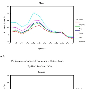
Figure 1

Performance of Adjusted Enumeration District Totals By Hard To Count Index

Males

Age Group

85+ 80-84 45-79 40-44 35-39 30-34 25-29 20-24 15-19 10-14 5-9 0-4

Root Mean Squar

e Er

ro

r

2.5

2.0

1.5

1.0

.5

0.0

HtC Index

Very Easy

Easy

Medium

Hard

Very Hard

Figure 2

Performance of Adjusted Enumeration District Totals

By Hard To Count Index

Females

Age Group

85+ 80-84 45-79 40-44 35-39 30-34 25-29 20-24 15-19 10-14 5-9 0-4

R

oot

M

ean Square Error

2.5

2.0

1.5

1.0

.5

0.0

HtC Index

Very Easy

Easy

Medium

Hard

Very Hard

From Figures 1 and 2 it can be seen that even for the hardest to count group males for the RMSE stays between 1 and 2. This represents an error of between 1 and 2 people on average across the enumeration districts as a result of variability and bias. For other groups it is below 1. It is of use to see the bias on its own as this can seriously effect confidence interval coverage if it dominates the variance. In reality it is non-trivial, if not impossible, to estimate the bias as the true value is not known. Figures 3 and 4 present the bias for males and females.

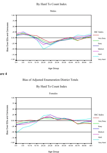
Figure 3

Bias of Adjusted Enumeration District Totals

By Hard To Count Index

Males Age Group 85+ 80-84 45-79 40-44 35-39 30-34 25-29 20-24 15-19 10-14 5-9 0-4 Bias Ov er ED

s and C

ens us es 1.00 .75 .50 .25 0.00 -.25 -.50 -.75 -1.00 HtC Index Very Easy Easy Medium Hard Very Hard Figure 4

Bias of Adjusted Enumeration District Totals

By Hard To Count Index

Females Age Group 85+ 80-84 45-79 40-44 35-39 30-34 25-29 20-24 15-19 10-14 5-9 0-4 Bi as Ov er ED

s and C

9.2 The bias shows a slightly different picture. As expected 20-34 year old males are being systematically underestimated but the comparing the bias to the RMSE in figure 1 shows that it is not dominating the overall performance. What is less expected is the strong negative bias for 0-4 year old females compared to the only slight positive bias for males of the same age, when the RMSE in each case is similar. This shows that the bias for the females is having a comparatively larger effect on the RMSE than it is for the males.

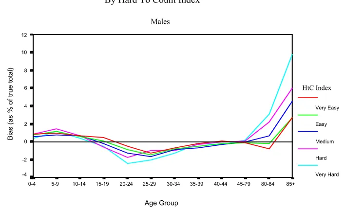
From the absolute size of the bias, the worst case is that on average ½ a 0-4 year old female and ½ a 20-24 year old male are missed for each very hard to count enumeration district. Showing the relative bias puts these and the other biases into context as a proportion of the total number of people you are trying to estimate. The relative biases are presented in Figures 5 and 6.

Figure 5

Relative Bias of Adjusted Enumeration District Totals

By Hard To Count Index

Males Age Group 85+ 80-84 45-79 40-44 35-39 30-34 25-29 20-24 15-19 10-14 5-9 0-4 Bi as (a

s % o

f tru e to ta l) 12 10 8 6 4 2 0 -2 -4 HtC Index Very Easy Easy Medium Hard Very Hard Figure 6

Relative Bias of Adjusted Enumeration District Totals

By Hard To Count Index

Females Age Group 85+ 80-84 45-79 40-44 35-39 30-34 25-29 20-24 15-19 10-14 5-9 0-4 B ia s ( a s % o f tr u e to ta l) 12 10 8 6 4 2 0 -2 -4 HtC Index Very Easy Easy Medium Hard Very Hard

Figure 7

Performance of Adjusted Enumeration District Totals

Relative to Unadjusted Census Totals

Males and HtC = 'Very Hard'

Age Group

85+ 80-84 45-79 40-44 35-39 30-34 25-29 20-24 15-19 10-14 5-9 0-4

R

oot

Mean S

quare E

rror

5

4

3

2

1

0

Adjusted Count Census Count

Figure 8

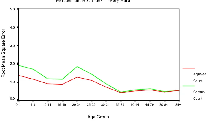
Performance of Adjusted Enumeration District Totals Relative to Unadjusted Census Totals

Females and HtC Index = 'Very Hard'

Age Group

85+ 80-84 45-79 40-44 35-39 30-34 25-29 20-24 15-19 10-14 5-9 0-4

R

oot

Mean Square Error

5.0

4.0

3.0

2.0

1.0

0.0

Adjusted

Count

Census

Count

missed but no overcount is simulated. However, for the adjusted counts, the bias is averaged over positive and negative quantities.

Figure 9

Bias of Adjusted Enumeration District Totals Relative to Unadjusted Census Totals

Males and HtC Index = 'Very Hard'

Age Group

85+ 80-84 45-79 40-44 35-39 30-34 25-29 20-24 15-19 10-14 5-9 0-4

Bi

as

O

ver

EDs

and Cens

us

es

1

0

-1

-2

-3

-4

Adjusted

Count

Census

Count

Figure 10

Bias of Adjusted Enumeration District Totals Relative to Unadjusted Census Totals

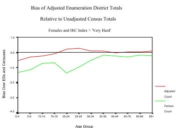
Females and HtC Index = 'Very Hard'

Age Group

85+ 80-84 45-79 40-44 35-39 30-34 25-29 20-24 15-19 10-14 5-9 0-4

Bi

as

O

ver

EDs

and Cens

us

es

1.0

0.0

-1.0

-2.0

-3.0

-4.0

Adjusted

Count

Census

Count

enumeration districts, and higher adjustments to 20-34 year olds. It will also slightly raise adjustments for 0-4 year olds and 85+. As there are only fixed effects, the model will give too much to young males (the sex effect) and not enough to young females. For the oldest age group, males are relatively unimportant as there are so few males in the 85+ group. The females dominate and push the age adjustments up; adding the sex and index effects leads to the positive bias for males. (This is seen best on the relative bias charts (Figures 5 and 6) where the small numbers in the denominator make the small biases relatively more different.) However, while the age adjustment for females might push the adjustments up, the sex effect pushes it down. This leads to negative bias for most index groups, except for the very hard to count group where the index effect is too strong.

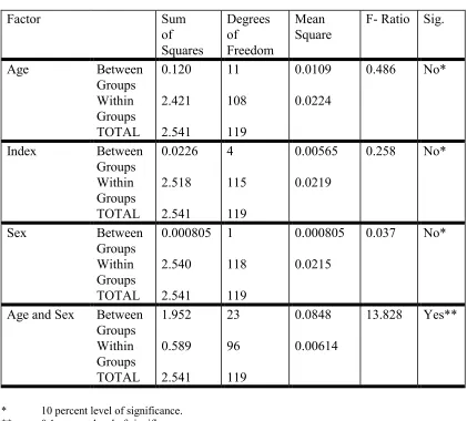
9.7 To investigate this further, a one-way ANOVA was performed on the bias using age groups, sex, and index as the factor. It was also carried out for age sex groups combined.

Table 1 - ANOVA for the Adjusted Count Bias

Factor Sum

of Squares

Degrees of Freedom

Mean Square

F- Ratio Sig.

Age Between

Groups Within Groups TOTAL

0.120

2.421

2.541

11

108

119

0.0109

0.0224

0.486 No*

Index Between

Groups Within Groups TOTAL

0.0226

2.518

2.541

4

115

119

0.00565

0.0219

0.258 No*

Sex Between

Groups Within Groups TOTAL

0.000805

2.540

2.541

1

118

119

0.000805

0.0215

0.037 No*

Age and Sex Between Groups Within Groups TOTAL

1.952

0.589

2.541

23

96

119

0.0848

0.00614

13.828 Yes**

* 10 percent level of significance. ** 0.1 percent level of significance.

factor in a one-way ANOVA suggesting that an age-sex interaction would improve the model and reduce the variation in the bias for certain specific groups.

10. Conclusions and Further Work

10.1 These initial results are promising and show that the method works. The model is a simple fixed main effects model. The one-way ANOVA results combined with the shape of the female bias suggest that interacting sex with certain age groups (0-4, 20-34, 85+) will improve results for both males and females. In the reality of the One Number Census one would also expect to do even better by fitting random effects to account for additional small area variability. (Random effects have not been fitted yet as the current simulation has no small area variability beyond enumeration districts belonging to the same hard to count group.) These results are obtained by using 1/π0 to adjust for all missing people. The next stage is to do a similar analysis for the π1 /π0 and π2 /π0 adjustments for this simple model using the standard simulation.

10.2 The models were fitted using SAS which handles the situation where certain response groups do not exist and gives a warning. SAS effectively sets the value of the parameters to negative infinity, which results in predicted probabilities of approximately zero. Once models are required with random parameters it is necessary to use MLn (a multilevel modelling computer package) or some similar package. The same result can still be achieved by using the offset command to set parameters and thus stop MLn from trying to fit them.

10.3 To investigate more complex models requires a more complex simulation. The current simulation only excludes people from the Census based on age, sex and HtC index, hence these are the only variables the multinomial model uses. The next two major steps are to include household structure into the model and then extend the simulation model. Extending the simulation model will include using other variables to exclude people such as economic status, ethnicity and tenure. It will also involve introducing spatial small area effects into the data. This will allow us to investigate how strong these small area effects need to be for the fixed effects estimation model not to be sufficient and need random effects. It will also allow investigation into the value of the spatial smoothing of random effects that has been proposed. There is also the need to do sensitivity analysis of the models to dependence between the Census and CCS as well as CCS undercoverage.