Marine Geophysical Researches 20: 13–20, 1998.
© 1998 Kluwer Academic Publishers. Printed in the Netherlands. 13
Optimal Processing of Marine High-Resolution Seismic Reflection (Chirp)
Data
R. Quinn
1,∗, J. M. Bull
1& J. K. Dix
2Departments of Geology1and Oceanography2, Southampton Oceanography Centre, University of Southampton, Southampton SO 14 3ZH, U.K.
Received 15 August 1997; accepted 1 July 1998
Key words: Chirp, processing, source-signature, high-resolution seismic
Abstract
Chirp frequency-modulated (FM) systems offer deterministic, repeatable source-signatures for high-resolution, normal incidence marine seismic reflection data acquisition. An optimal processing sequence for uncorrelated Chirp data is presented to demonstrate the applicability of some conventional seismic reflection algorithms to high-resolution data sets, and to emphasise the importance of a known source-signature. An improvement of greater than 60dB in the signal-to-noise ratio is realised from correlating the FM reflection data with the transmitted pulse. Interpretability of ringy deconvolved data is enhanced by the calculation of instantaneous amplitudes. The signal-to-noise ratio and lateral reflector continuity are both improved by the application of predictive filters whose effectiveness are aided by the repeatability of the Chirp source.
Introduction
Chirp sub-bottom profilers are high-resolution frequency-modulated marine sources offering vertical resolution on the decimetre scale in the top c. 30 m of unconsoli-dated sediments. The vertical resolution of Chirp sys-tems is dependent upon the bandwidth of the source; e.g. the 2–8 kHz source used in this study equates to a theoretical vertical resolution of 0.125 m (assuming a compressional wave velocity of 1500 m s−1). The horizontal resolution of Chirp systems is primarily de-pendent upon the source characteristics (beam angle, dominant frequency), compressional wave velocity of the sediments, towfish altitude and pulse rate of the system; with characteristic horizontal resolutions of 1 to 2 m. Typical applications of Chirp systems in-clude marine bottom-sediment classification, marine foundation, pipeline laying, platform and well-site evaluation, and archaeological and environmental im-pact surveys (see Bull et al., 1998, for a typical case study).
∗Now at: School of Environmental Studies, University of Ulster, Coleraine BT52 1SA, Co. Derry, Northern Ireland.
The principle feature that distinguishes Chirp sys-tems from short-pulse, single-frequency profilers (e.g. boomers and pingers) is the nature of the Chirp source-signature. The sonar system transmits computer-generated, swept- frequency pulses (Figure 1a) which are amplitude- and phase-compensated (Schock et al., 1989; LeBlanc et al., 1992a; Panda et al., 1994). This precise waveform control helps suppress source-ringing which is a common problem affecting the vertical resolution of short-pulse profilers. In addition, the Chirp waveform is weighted in the frequency do-main to possess a Gaussian spectrum (Figure 1b). The autocorrelation of the Chirp pulse is the zero-phase Klauder wavelet shown in Figure 1c.
Figure 1. (a) The 32 ms frequency-modulated Chirp pulse linearly
[image:2.595.312.523.64.441.2]sweeping from 2–8 kHz. (b) Power spectrum of the Chirp pulse. (c) Klauder wavelet – the autocorrelation of the Chirp pulse.
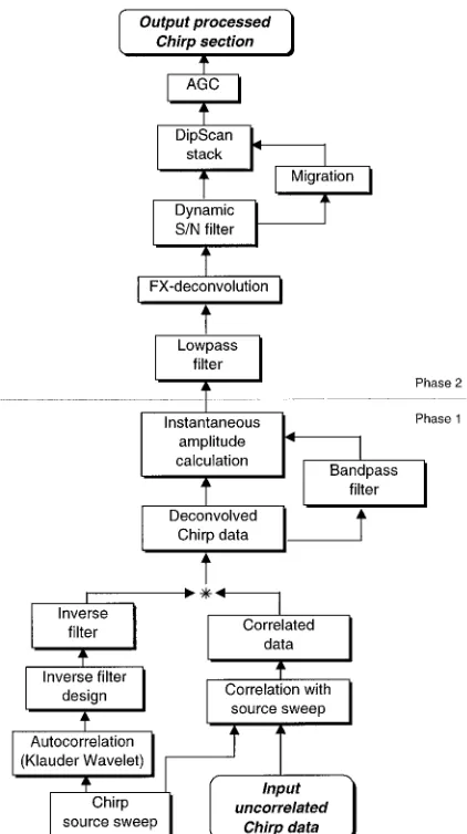
Figure 2. Flow chart showing the processing sequence applied to
uncorrelated Chirp data. Phase 1 = correlation and deconvolution; Phase 2 = filtering.
quantitative sediment analysis. Results indicate that the application of predictive filter techniques to Chirp sub-bottom data is successful in increasing both the signal- to-noise ratio (SNR) and the lateral continuity of the data.
Methodology
[image:2.595.82.279.106.602.2]15
Chirp (Figure 1) pulse of bandwidth 6 kHz (sweep of 2–8 kHz) with a repeat period of 250 ms and a sample interval of 40µs was employed. The carrier frequency (or central frequency), fc, of this pulse is 4.6 kHz (Figure 1b). Swell filters were not employed during data acquisition.
The Chirp section examined in this paper rep-resents a continuous, single-channel profile of 200 traces, with an average trace-interval of 0.6 m ac-quired in an average water depth of 7.5 m. All data processing was conducted in the software package ProMAXTM 6.0 (Advance Geophysical Corporation) mounted on a SUN Ultra workstation. Processing al-gorithm and parameter suitability were assessed by their effects on both single- and multi-trace Chirp seismograms. Processing of the uncorrelated data is divisible into two phases (Figure 2): (1) correlation and deconvolution and (2) filtering.
Two methods are employed to demonstrate the ef-fects of the processing algorithms on the uncorrelated data. The first method is the presentation of the full profile at significant stages within the processing se-quence. The second mode of display is single-trace seismograms (together with associated power spectra) in which the effects of each step in the processing sequence can be examined in detail. Trace 3100 is chosen as the display trace as it possesses a relatively low SNR and the effects of each processing stage can be readily appreciated (Figure 3).
Chirp Data Processing
Phase 1 – Correlation and Deconvolution
A zero-phase correlation of the uncorrelated data was performed utilising the source sweep in Figure 1a. The resulting correlated data are effectively the superposi-tion of the Klauder wavelet (Figure 1c) on the earth’s impulse response, plus some noise component. The results of correlation with the source sweep are illus-trated in the profile of Figure 4 and the single-trace seismogram of Figure 5a. In the complete profile, the major reflection events (seabed at 10 ms and bedrock profile between 20 and 25 ms) are distinguishable, but sharp detail in the sediment pile is lacking due to the ringiness of the Klauder wavelet. However, the corre-lation process has considerably reduced the magnitude of the side-lobes (compare the power spectra of Fig-ures 3 and 5a), increasing the overall SNR of the data and aiding interpretability. A noticeable characteristic
of the correlated data is the downshifting of the carrier frequency from 4.6 kHz in the source sweep to 4.2 kHz in the reflection data. A similar effect was recognised by LeBlanc et al. (1992b) and attributed to sediment attenuation causing the centre frequency of the Chirp pulse spectrum to shift to a lower frequency.
Subsequent to correlation, a source-signature de-convolution (Figure 2, Phase 1) is performed to reduce the ringiness of the correlated data. The solution to the deconvolution problem is said to be determinis-tic (Yilmaz, 1987) as the Chirp source-signature is known exactly. An inverse filter (the inverse of the source autocorrelation) is calculated and this operator is convolved with the correlated data. A comparison of the correlated and deconvolved seismograms in Fig-ures 5a and 5b demonstrates that individual reflectors are enhanced by this process, and previously indistin-guishable events are revealed. However, this process fails to convert the seismogram into a series of pure spikes representing the desired impulse response, and the data still suffers from ringiness and lacks defini-tion. The success of deconvolution is possibly limited by the presence of noise in the reflection data and reflection composites caused by the constructive and destructive interference of closely spaced reflectors.
In order to increase the interpretability of the de-convolved Chirp data, the instantaneous amplitude (a measure of the reflectivity strength),R(t), of the sig-nal is calculated. R(t)is proportional to the square root of the total energy of the seismic signal at an instant in time (Yilmaz, 1987):
R(t)=sqrtx2(t)+y2(t), (1)
Figure 3. Single uncorrelated Chirp seismogram (Trace 3100) with associated power spectrum.
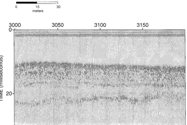
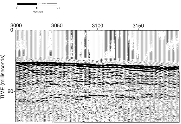
Figure 4. Correlated Chirp profile of 250 traces with an average trace interval of 0.6 m. The seabed and bedrock reflectors are imaged at
approximately 10 ms and 23 ms two-way travel time respectively.
Phase 2-filtering
The principal aims of the second phase in the process-ing sequence are to increase the overall SNR by the application of predictive filters and to enhance the lateral coherency of the data. The output from the in-stantaneous amplitude calculation is initially lowpass filtered to remove the high-frequency noise component (Figure 7a).
Subsequently, the Frequency-distance (FX-) de-convolution algorithm Fourier transforms each input trace, applies a Wiener prediction filter (in distance) for each frequency in the 20–2200 Hz range and then inverse transforms the data back to the time domain (Figure 7b). The operator is used to predict the sig-nal one trace ahead across the frequency slice and any difference between the predicted waveform and the ac-tual one is removed (Canales, 1884; Gulunay, 1986). In practice the Wiener filter is run in one direction and
subsequently run in the opposite direction to reduce prediction errors.
As a final stage in the filtering process, the FX-deconvolved data are passed through a dynamic signal-to-noise (SN) filter (20–2000 Hz, Figure 7c). This process eliminates the requirement of a time-variant bandpass filter design (and application) which is difficult to design with the relatively small data win-dow of the Chirp data (typically 10–40 ms for the 32 ms Chirp pulse). Additionally, this process en-hances the lateral coherency of data by weighting each frequency-derived function from the local SNR by
weight(f )= S(f ) 2
S(f )2+N(f )2, (2)
where S is the predicted signal and N the noise component (ProMAXT M 6.0 User Manual). Unlike conventional coherency enhancing methods such as
trace-mixing and FX-deconvolution, this process does
[image:4.595.145.461.190.401.2]ap-17
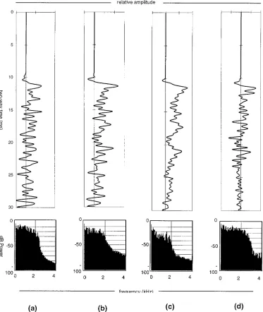
Figure 5. Diagram illustrating the initial 3 stages in the processing history of the Chirp profile. Single-trace seismograms (Trace 3100) are on
top and their associated power spectra are shown below. (a) Zero-phase correlation (b) Source- signature deconvolution of 5a (c) Instantaneous amplitude correction applied to 5b. See main text for more discussion.
[image:5.595.141.460.418.643.2]Figure 7. Diagram illustrating the latter 4 stages in the processing history of the Chirp profile. Single-trace seismograms (Trace 3100) are on
top and their associated power spectra are shown below. (a) Bandpass filtered 5c (b) FX-deconvolution of 7a (c) Dynamic SN filter of 7b (d) Dip-scan stack of 7c.
plied as an amplitude-only convolutional filter to each individual trace in turn and does not include a portion of neighbouring traces.
The final processing step is the application of the dip scan stack (see Yilmaz, 1987, for discussion) algorithm to enhance coherent seismic events by a weighting process. This algorithm transforms the in-put time-domain profile into a user defined range (in this case±0.18 ms per trace) of dip stacked traces.
19
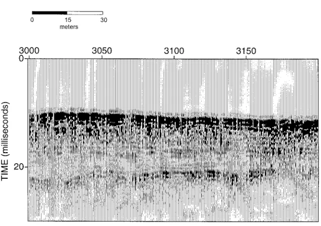
Figure 8. Final processed Chirp profile.
a cleaner and more interpretable profile. Although the final profile of Figure 8 has been converted to instantaneous amplitude earlier in the processing his-tory, the section appears to possess polarity informa-tion. However, this negative component is attribut-able to additive effects caused by the application of the coherency-enhancing filters discussed above, and must not be interpreted as real events. Close compar-ison between Figures 6 and 8 and knowledge of local geology (West, 1980) indicate the coherent reflection events in the final processed section are real events and not processing artefacts.
Conclusions
Correlation and deconvolution of Chirp data are greatly facilitated by detailed knowledge of the source-signature. An improvement of greater than 60dB in SNR is realised from correlating the FM reflected data with the transmitted pulse. Effective deterministic deconvolution is accomplished by de-signing an inverse filter based on the autocorrelation of the source waveform to produce the Klauder wavelet. Interpretability of the Chirp profile is further aided by the calculation of the instantaneous amplitude which smoothes the ringy appearance of the deconvolved data in time.
SNR and reflector continuity are enhanced by the application of a series of predictive filters. The ef-fectiveness of these coherency enhancing methods
benefits from the repeatability of the source pulse, as the frequency content of the signal remains rela-tively constant throughout the correlated profiles, and is therefore readily distinguishable from any arbitrary noise component.
Acknowledgements
The authors thank the following: GeoAcoustics Ltd., Great Yarmouth, U.K. for permission to publish the Chirp pulse; Dr. Tim Minshull, Bullard Labs, Cam-bridge University for helpful discussion. Data was acquired utilising a GeoAcoustics GeoChirp Model 136A towed transducer system. This research was funded by NERC Grant GR3/9533.
References
Advance Geophysical Corporation, 1995, ProMAXT M 6.0 User Manual.
Bull, J. M., Quinn, R., and Dix, J. K., 1998, Reflection coeffi-cient calculation from marine high-resolution seismic reflection (Chirp) data and application to an archaeological case study:
Marine Geophysical Researches 20, 1–11.
Canales, 1984, Random noise reduction. Paper presented at the Society of Exploration Geophysicists 54th Annual Conference, Atlanta, GA.
LeBlanc, L. R., Panda, S., and Schock, S. G., 1992a, Sonar attenu-ation modeling for classificattenu-ation of marine sediments, J. Acoust.
Soc. Am. 91, 116–126.
LeBlanc, L. R., Mayer, L., Rufino, M., Schock, S. G. and King, J., 1992b, Marine sediment classification using the chirp sonar: J.
Acoust. Soc. Am. 91, 107–115.
Panda, S., LeBlanc, L. R., and Schock, S. G., 1994, Sediment classification based on impedance and attenuation estimation, J.
Acoust. Soc. Am. 95, 3022–3055.
Schock, S. G., LeBlanc, L. R. and Mayer, L. A., 1989, Chirp sub-bottom profiler for quantitative sediment analysis, Geophysics 54, 445–450.
West, I. M. (1980) Geology of the Solent Estuarine System, In: The Solent Estuarine System: An assessment of present knowledge,
NERC Pub. Series C 22, 6–17.