Explaining the output of ensembles on a case by case basis

LEABHARLANN CHOLAISTE NA TRIONOIDE, BAILE ATHA CLIATH TRINITY COLLEGE LIBRARY DUBLIN OUscoil Atha Cliath The University of Dublin

Terms and Conditions of Use of Digitised Theses from Trinity College Library Dublin

Copyright statement

All material supplied by Trinity College Library is protected by copyright (under the Copyright and Related Rights Act, 2000 as amended) and other relevant Intellectual Property Rights. By accessing and using a Digitised Thesis from Trinity College Library you acknowledge that all Intellectual Property Rights in any Works supplied are the sole and exclusive property of the copyright and/or other I PR holder. Specific copyright holders may not be explicitly identified. Use of materials from other sources within a thesis should not be construed as a claim over them.

A non-exclusive, non-transferable licence is hereby granted to those using or reproducing, in whole or in part, the material for valid purposes, providing the copyright owners are acknowledged using the normal conventions. Where specific permission to use material is required, this is identified and such permission must be sought from the copyright holder or agency cited.

Liability statement

By using a Digitised Thesis, I accept that Trinity College Dublin bears no legal responsibility for the accuracy, legality or comprehensiveness of materials contained within the thesis, and that Trinity College Dublin accepts no liability for indirect, consequential, or incidental, damages or losses arising from use of the thesis for whatever reason. Information located in a thesis may be subject to specific use constraints, details of which may not be explicitly described. It is the responsibility of potential and actual users to be aware of such constraints and to abide by them. By making use of material from a digitised thesis, you accept these copyright and disclaimer provisions. Where it is brought to the attention of Trinity College Library that there may be a breach of copyright or other restraint, it is the policy to withdraw or take down access to a thesis while the issue is being resolved.

Access Agreement

By using a Digitised Thesis from Trinity College Library you are bound by the following Terms & Conditions. Please read them carefully.

Explaining The Output Of Ensembles

On A Case By Case Basis

Robert Wall

A thesis subm itted to the University of Dublin

for the degree of Doctor in Philosophy

^ T R \n n ycollege

^

D eclaration

T h e work descril^ed in this thesis is, except where otherwise sta te d , entirely t h a t of th e a u th o r and has not been s u b m itte d as an exercise for a degree a t this or any oth e r university.

Signed: Rol>ert Wall

P erm ission to Lend or C opy

I agree t h a t T rinity College L ibrary may lend or co{)y this thesis up o n request.

Signed: R o b e rt W^all

A cknow ledgem ents

I would like to acknowledge the heij) and s u p p o rt of num erous j^eoj^le d u rin g th e research and w riting of this thesis:

• My friends inside and outside of college, in p articular, Gabriele, C onor and my girlfriend D eborah.

• iMy nnnn, dad, sister and b ro th e r for their encouragem ent.

• D octors P aul Walsh and Stephen Byrne for th e essential work of analysing my results w ith o u t which this thesis would not have been j)ossible.

• D e p a rtm e n t of C o m p u te r Science, Trinity College for its financial s u p ­ p o r t ovc’r the last three years.

Sum m ary

T h i s tliesis in tr o d u c e s a novel m e t h o d for e x p la in in g th e p r e d ic tio n s o f e n ­ se m b le s o f artificial n e u ra l n e tw o rk s on a case liy case l)asis. C u r r e n t r e s e a rc h is ])riniarily d ire c te d to w a rd s b u ild in g global m o d e l, t h a t is, m o d e ls t h a t fully d e s c r ib e all possible i n p u t c o n d itio n s a n d th e i r a s s o c ia te d o u t p u t s . T h e a l t e r ­ n a ti v e case by case ajJi)roach is referred to as local e x p la n a ti o n . This thesis d e m o n str a te s a 'process for p erfo rm in g local explanation.

T h e c u r r e n t global a p p r o a c h is con sid e red ineffective d u e to a n im p lic it t r a d e oH' t h a t n u ist ta k e place d u r in g its c re a tio n . T h e t r a d e off is l)etw eeu t h e c o m p r e h e n s ib ility of th e rules a n d th e i r fidelity to th e o rig in a l e n s e m ­ ble i)redictions. In a d o m a i n w ith p o o r coverage, th is t r a d e of!' m ig h t be p a r t i c u l a r l y d e tr i m e n ta l .

In order to test th e perform auce and feasibility of th e system, th e k)cal ex])lanation process and rule ranking techniques were im])lemented in code. Ensem bles w ith backi)ropagation neural networks [50] as m em bers were used as tlie black box to be explained. T h e e x p lan ato ry rules were gen era ted using th e c4.5rules package [47]. B ackpropagation ensembles a n d c4.5rules are n ot th e only possibilities, and oth e r m e th o d s are also presented in th e background chapters.

Tw o d a ta se ts were used during testing and an exp ert in each do m a in eval­ ua te d th e results. B oth d a ta se ts were from the medical dom ain. T h e first d a ta s e t involved the j^rediction of which children disj^laying signs of bronchi­ olitis should l)e a d m itte d overnight to hospital. T h e second d a ta s e t involved the i^rediction of the W arfarin dosage to be adm inistered to i)atients based on th eir i)rtn-ious history of tak in g the d ru g and th eir curren t symijtoins. Th(' bronchiolitis d a ta s e t represented j)00rer coverage of its do m a in th a n the \\'a rfa rin d atase t.

C on ten ts

1

In tr o d u c tio n

12

1.1 Coiitrii)utions of this T h e s i s ... 16

1.2 S tru c tu re of T h e s i s ... 16

2

N e u r a l N e tw o rk s

19

2.1.1 S tru c tu re ... 20

2.1.2 T r a i n i n g ... 23

2.1.3 Execution - - Steps 3 - 5 ... 28

2.1.4 Training — Steps 3 9 ... 28

2.2 Considerations when Training Neural Networks ... 29

2.2.1 O v e r f i tt in g ... 29

2.2.2 Bias & Variance in Neural Networks ... 31

3

E n sem b le s

33

3.1.1 B a g g i n g ... 36

3.1.2 B o o s t i n g ... 36

3.1.3 Cross Validation E n s e m b l e s ... 38

3.1.4 F eature S u b s e t s ... 38

3.2.1

A v e r a g i n g ...

3.2.2

Linear R e g re s s io n ...

3.2.3

Principal Components R e g r e s s i o n ...

3.3

Summary ...

4

R u le L ea rn in g A lg o r ith m s

4.1

Decision T r e e s ...

4.1.1

C 4 . 5 ...

4.1.2

Classification and Regression Trees ( C A R T ) ...

4.1.3

Rule Extraction from Decision T r e e s ...

4.2

Rule Inducing Algorit h m s ...

4.2.1

C N 2 ...

4.2.2

F O I L ...

4.2.3

R I P P E R ...

4.2.4

S L I P P E R ...

4.3

Summary ...

5 E x p la in in g N eu ra l N etw o rk s

5.1

Strategies ...

5.1.1

Network Decomposition ...

5.1.2

Black B o x ...

5.2

Evaluating Rule Q u a l i t y ...

5.3

Global V Local E x i ) l a n a t i o n ...

5.4

Rule Extractions from E n s e m b l e s ...

5.5

Summary ...

6 S o lu tio n

G.l

Building an Ensemble of Rules from an Ensemble of Neural

N e tw o rk s...

6.2

Rule Coverage S t a t i s t i c s ... 90

6.2.1 Advanced Rule Coverage S t a t i s t i c s ... 91

6.2.2 Rule Fit and Ranking ... 91

6.2.3 Worked Example of Calculating Rule Fit Using Iris

Dataset ... 94

6.3

Rule S im p lif ic a tio n ... 97

7

I m p le m e n ta tio n

99

7.1

I n t r o d u c t i o n ... . 99

7.2

Practical Implementation I s s u e s ... 99

7.2.1 P r o g r a m m i n g ... 99

7.2.2 Distributing Work

... 101

8

E v a lu a tio n

104

8.1

Evahuition P r o c e s s ... 105

8.2

B ronchiolitis... 108

8.2.1

D a t a ...108

8.2.2 Exi)lanations ... 109

8.3

W 'a rfa rin ... I l l

8.3.1

D a t a ...I l l

8.3.2 Ex])lanations ... 112

8.4

Suiiniiary ...114

9

C o n c lu sio n s & F u ture W ork

122

9.1

Future W o r k ... 124

List o f F igures

2.1 Single layer neural n e t w o r k ... 21

2.2 G ra p h of logical X O R f u n c t i o n ... 22

2.3 M ultilayer hackpropagation neural n e t w o r k ...26

2.4 G ra p h of train in g and generalisation error ... 30

4.1 E xam ple decision tree using Iris d a t a ... 46

4.2 D a ta t h a t is ill suited for decision tree le arn in g ...47

4.3 E x am ple rules extra cted from the decision tree in Figure 4.1. 59 4.4 CN2 algorithm ... 61

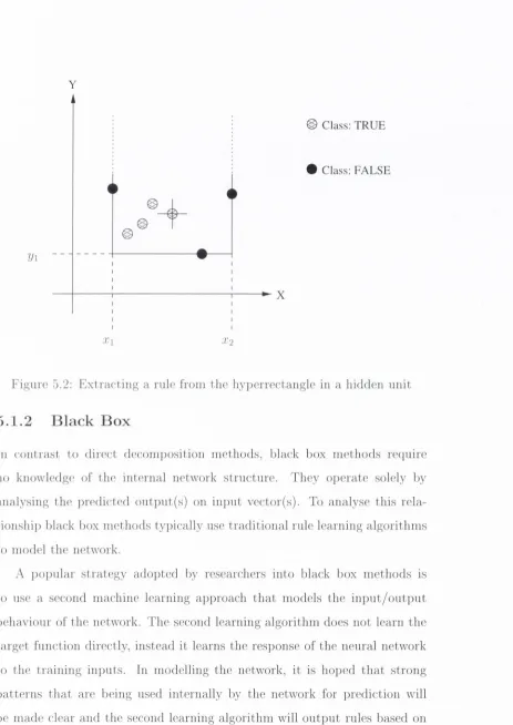
5.1 Shrinking th e dimension of a rectagle in rectan g u lar basis func­ tion n e t w o r k s 74 5.2 E x tra c tin g a rule from the hyi)errectangle in a hidden u n it . . 75

6.1 N u m b er line showing unbounded r u l e ... 93

6.2 Grai)h of Iris d a t a in two d i m e n s i o n s ... 96

List o f Tables

2.1 XOR t r u t h table ... 21

4.1 E rrors before and after rule ])runing in C 4 . 5 ... 57

8.1 Bronchiolitis d a ta se t s t r u c t u r e ... 108 8.2 Results of 5-fold cross validation performed on bronchiolitis datalOO 8.3 Bronchiolitis example evaluated by expert ... 110 8.4 Rules produced for the exam ple in Table 8 . 3 ...117 8.5 Accuracies on test d a t a ... 118 8.6 W ins, losses and draws for the rules com p u ted by the local

('xplanation m e t h o d ... 118 8.7 Analysis of rules generated for bronchiolitis d a t a ...118 8.8 W arfarin d a ta s e t s t r u c t u r e ... 118 8.9 Results of 5-fold cross validation perform ed on W arfarin d a t a . 118 8.10 W arfarin exam ple evaluated by expert ... 119 8.11 Rules produced for the exam ple in Table 8.10 ... 120 8.12 Accuracies on test d a t a ... 121 8.13 W ins, losses and draws for the rules com puted by th e local

e x p lan atio n m e t h o d ... 121 8.14 Analysis of rules generated for th e W arfarin d a t a ...121

C hapter 1

In trod u ction

T h e i)reclictioii accuracy of neural networks and in i)articnlar neural network ensembles has improved, as a result of recent research, to th e point t h a t th e y frefjuently outp e rfo rm m any tra d itio n a l systems. Desi)ite this im provem ent, their ado])tion as a useful prediction tool in m any areas has been slow to non existent.

"ilie reasons for this j)oor utilisation in the field of medical diagnosis, a lth o u g h the reasons are similar for other fields, is sum m arised in this in­ tro d u c tio n and fu rth er expanded th ro u g h o u t the thesis. T his in tro d u c tio n also provides an overview of how the research described in this thesis can overcome these difficulties.

Medical d a ta se ts provide one of th e richest sources of prediction prol)- lems ideally suited to prediction techniques. Medical staff could benefit enor­ mously from system s t h a t could assist th e m in diagnosing and u n d e rs ta n d in g medical problems.

as people in general are wary of tru stin g any prediction (either from people or com puters) w ith o u t an explanation. In addition, the p resen ta tio n of a diagnosis in such a definitive form by neural netw'orks could lead th e do cto r to feel t h a t h is /h e r role is being u nderm ined or even usurj^ed. P roviding an exi)lanation of th e o u tp u t m ight improve confidence in th e i^redictive cai)abilities of the system thus ensuring greater user acceptance.

In a m ore general context, the problem of lack of ex planation m ay be even m ore critical. For instance, use of a neural network in a u t o m a te d safety critical tasks m ay be impossible, if operatioti of th e network ca n n o t l)e veri­ fied.

To achieve the goal of using neural networks in medical research it is therefore necessary to:

• Take advantage of ensembles of neural networks to provide i)redictions t h a t are as accurate as possible.

• Provide comi)rehensible explanations for the user of th e o u tp u t of the ensemble.

• P resent exi)lanations to the user, such as a d octor or oth e r iHofessioual user, in such a way t h a t th e inform ation presented m ay be used to com plem ent h is /h e r ])rofessional experience and ju d g e m e n t and n o t to replace it.

T his thesis addresses each of these issues in tu rn and provides ])ossible solu­ tions.

M ost researchers have focused on producing models of an entire p h e ­ nomenon. These models will be referred to here as “global m odels” . T h e aim of these global models is to produce a com prehensible form t h a t p ro ­ vides ai)proi)riate o u tp u ts for all possible variations of inputs. T his ty p e of model is useful for explaining m any types of problems.

For exami)le, a doctor involved in providing “In V itro F ertilisation” (IV F) is more likely to be a specialist in this area. A global model can aid in th e d o c t o r ’s u n d e rs ta n d in g of the dom ain to the fullest extent by s u m m a risin g all of th e conditions under which IV F will be successful or unsuccessful. T h e global model m ay also help provide new insights into th e dom ain. F u rth e r­ more, th e global model may helj) doctors allocate scarce hospital resources to those cases where they will be of m ost benefit.

In ])ro(lucing these models, there is an im plicit trade-off between co m p re­ hensibility and fidelity:

• Coniprehtmsihility is an estim atio n of th e u n d e rs ta n d a b ility of the model.

• Fidelity is a m easure of how closely the derived model predicts the sam e o u tp u ts as the the original model.

Simplifying a complex model (e.g. by prun in g a decision tree) to make it m ore com prehensibile may result in a loss of fidelity, i.e. th e derived m o d e l’s capacity to exj)lain the original network diminishes.

An exam ple of a s e ttin g like this would be th e busy accident and em e r­ gency w ard of a hospital. D octors here are concerned w ith th e quick diagncxsis of p a tie n t s y m p to m s and less w ith the m im itiae of a problem dom ain. In this situ a tio n , alternatives to a global model m ay be more useful.

T h e a ltern ativ e aj)proach will be referred to as local explanation. Local ex p lan atio n can be seen as on-dem and explanation. For each individual p rediction m ade by the ensemble a tailored ex planation is produced t h a t b est exi)lains it in term s of the in p u t features. Delaying th e p ro d u ctio n of an ex p la n a tio n like this allows th e system to use all available d a t a for every prediction. Tailoring the explanation according to the symj)toms displayed ensures t h a t th e m ost a p p ro p ria te explanation is o u tp u t.

T h is thesis takes the approach of displaying a nimiber of j)Ossible expla­ natio n s in order to ensure t h a t these local explanations act to com plem ent th e d o c t o r ’s reasoning.

global model can only provide a single explanation. T his exi)lanation may fail to cai)ture all of th e details of the prediction. This could be due to th e com p re h en sib ility /h d elity tra d e off encountered in its p roduction. If there is m ore th a n one regularity in the d a t a t h a t exj^lains this prediction th e glol)al model may also fail to show this.

T h e local exjilanation approac:h of displaying several rules a t once, over­ comes these difficulties. Because tlie rules explaining th e prediction are n ot chosen until the last m om ent no details are lost as a result of com prehensibil- it y /h d e l ity trade-offs. Also, the approach of displaying several rules a t once m eans t h a t different regularities explaining the prediction t h a t were c a p tu re d from th e diverse ensemble m em bers (th a t correctly predicted the result) can also be dis])layed.

explana-tioiis th a n are to be displayed. To overcome this, the rules are ranked using a novel ranking technique developed as p a rt of this thesis. This technique allows rules to be selected as predictive w ith increased confidence even if th e coverage of t h a t rule on th e train in g d a t a is poor (this problem is often known as th e small disjunct problem [35]).

T h e d o c to r can now decide on th e validity behind the logic in each rule an d thus th e overall validity of tlie ensemble prediction itself.

1.1

C ontribu tions of this T hesis

T h e princij^al contriljutions of this thesis to an u n d e rs ta n d in g of explaining ensembles of neural networks are:

• D em o n strates a process for exi)laining o u tp u ts on a case by case basis.

• D em o n strates an evaluation of the case by case basis to explan atio n t h a t shows t h a t local explanation is of p a rtic u la r use when the d a t a coverage is j)oor.

• D e m o n strates and introduces a new m easure for determ in in g the fit of an exam ple to a rule.

• D e m o n strates t h a t a sul)set of rules ranked using th e calculated rule fit forms a concise and easily u n d ersto o d explanation.

1.2

Structure o f Thesis

C lia i)te r 2 e x p la in s b a c k p r o p a g a ti o n n e u ra l n e tw o rk s wdiich a re t h e n e t ­ works u sed in th e Iini^leinentation s e ctio n of th is th esis d u e to t h e i r p ro v e n tra c k re c o rd [58, 53] ( a lt h o u g h o t h e r n e tw o rk ty p e s co u ld also b e u s e d ). C h a p t e r 3 p r e s e n ts m e t h o d s for b o t h c r e a ti n g e n sem b le j^redictions a n d c o m - l)ining t h e m t o o b t a i n th e b e s t results.

T h e first h a lf of C h a p t e r 4 covers decision tre e a lg o r i th m s , w hile t h e second h a lf c o n c e n t r a t e s on a lg o r i th m s t h a t ca n lea rn rules directly. T h e purj)ose o f t h is cha[)ter is tw'ofold. Firstly, t h e m e t h o d chosen to e x p la in in d iv id u a l n e u ra l n e tw o rk s is to b u ild a m o re c o m p r e h e n s ib le le a rn e r, e.g. a decision tree, to m o d el th e n e u ra l netAvork by u sin g d a t a t h a t h a s b e e n l ab e lle d l)v th e netw ork. A n y of th e m e t h o d s p r e s e n te d in t h a t c h a p t e r c an be used to do this. Secondly, th e m e t h o d p ro p o s e d for th e e x p l a n a t i o n o f e n s em b les of n e u ra l n e tw o rk s ca n in fact be ge n e ra lis e d to e x p la in a n e n s e m b le of rules. T h e choice of which m e t h o d to use is left e n tire ly t o th e m o d elle r. T h i s choice could be g u id e d by p e rs o n a l preference, p e r f o r m a n c e on p a r t i c u l a r d a t a or a v a ila b ility of e x is tin g code or t im e to i m p l e m e n t a HK'thod (a m o d u l a r s y s te m could swaj) one ru le le a r n e r w ith a n o t h e r w i t h l it ll e t r o u b k ; la te r if re q u ired ).

C h a i ) t e r 5 looks a t e x is tin g s tr a te g ie s for e x p la in in g in d iv id u a l n e u r a l n e tw o rk s. T h i s cha])ter con c lu d e s w'ith a look a t w h a t l ittle rese a rc h h a s be('n d o n e to d a t e on th e i)roblem of e x p la in in g ensem bles.

C h a p t e r 6 ])resents a s o lu tio n to th e p r o b le m of e x p la n a ti o n , f o cu s in g on n e u ra l n e tw o rk s l)ut in c lu d in g a n o te on using p u r e rule b a s e d ensem bles.

C h a p t e r 7 o u tlin e s a b rie f d e s c r ip tio n of th e s o lu tio n i m p l e m e n ta t io n . C h a p t e r 8 in clu d e s a n e v a lu a tio n of th e m e t h o d in two d o m a i n s by e x p e r t s in each d o m a i n .

C hapter 2

N eural N etw orks

Artificial neural networks are developing rapidly in the field of m achine learn ­ ing. A lready they have d e m o n stra te d [58, 53] t h a t they generalise well for a b road a rray of b o th classification and regression problems. T h e fu n d a m e n ta l idea driving the develo])ment of neural networks is to model the o p eratio n of th e neurons in the l)rain.

Neural network units are interconnected by weights (similar in function to th e axon and dendrites in the brain). Firstly, th e to ta l signal received by a u n it is scaled and propag ated to all connected units. Secondly, th e signal reaches some outj)ut units t h a t trigger a physical reaction. T h e o u tp u t from a sim pler artificial neural network could similarly be used to control some reaction, e.g. in a robot, b u t more often the o u tp u t is sim ply o u tp u t te d for use by th e user.

S tep p in g up from their m ost basic stru c tu re , th e overall function of these u n its is to p a rtitio n the in p u t space into sep arate regions. T h e o u tp u t s tre n g th varies across regions and is either directly in terp reta b le in the case of regression j^roblems or can be rnajiped to a class for classification problems.

net,work, th e network can be train ed to api^roxiniate any contiinious function to any degree of accuracy [36]. In practice, however, this is rarely feasi­ ble. T h e d a t a available for tra in in g frequently represents only a subset of the entire function. In troducing m any more hidden units for tra in in g in­ volves tu n in g m any more im ram eters in th e network and these p ara m e te rs are likely to overfit the available d ata. By this it is m e an t t h a t th e network will lose its ability to generalise to new instances.

T h e power of neural networks comes w ith a heavy cost, however, their o p eratio n is cjuite opaciue. It is imi)ossible for even an experienced user to visualise the regions (hyperplanes in the case of backproi)agation neural networks) sep a ra tin g the different o utputs. N eural network oj)eration has a t ­ tra c te d the black box moniker for this oi)aque behaviour. C h a p te r 5 presents an overview of research t h a t tries to exj^lain th e predictions of neural n e t­ works.

Section 2.1 of this chapter will look a t backpro})agatiou neural networks. Some o th e r issues th a t m ust be taken into accotuit in neural netw'orks are discussed in Section 2.2.

2.1

B a ck p ro p a g a tio n N eu ra l N etw o rk s

2.1.1

Structure

S in g le L ayer N e tw o rk s

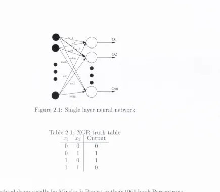
For simi)le learning tasks, it may be sufficient to use a single layer neural network. T h a t is w'here in p u t units are connected directly to a layer of o u tp u t units. Every in p u t neuron is connected to every o u tp u t neuron. A d ia g ra m of such a network is given in hgure 2.1

01 w 2.

02 w i l l )

w n2

Om

F ig u i'e 2.1: Single layer n e u ra l n e tw o rk

Table 2.1: X O R t r u t h ta b le ;ci O u tp u t

0 0 0

0 1 1

1 0 1

1 1 0

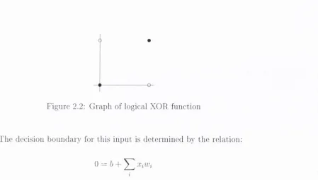
h ig h lig h te d d ra m a tic a lly by M in s k y & P a p e rt in th e ir 1969 b o o k P e rc e jjtro n s [42]. In th is boo k, th e y d e m o n stra te d th a t a single layer n eural n e tw o rk was in c a pa b le o f le a rn in g even the sim p le X O R lo g ic a l fu n c tio n . T h e p ro b le m is th a t th e class o u tp u ts o f th is fu n c tio n are n o t lin e a rly separable. T h e t r u t h ta b le fo r th is fu n c tio n is set o u t in ta b le 2.1 and th e p ro b le m o f s e p a ra b ility is easily seen in the d ia g ra m in figure 2.2. No single lin e can be d ra w n to separate th e o u tp u t classes.

In m a th e m a tic a l term s, th is p ro b le m can be seen as follow s. T h e re­ sponse o f th e o u tp u t o f a single layer n eural n e tw o rk is t j i n - T h is response is d e te rm in e d by th e in p u ts and the w eights c o n n e ctin g these in p u ts to th e

O U t ] ) U tS .

o

o

-F ig u re 2.2: G r a p h of logical X O R f u n c tio n

T h e decision l)o u n d a r y for th is i n p u t is d e te r m i n e d by t h e re la tio n ;

D e])ending on t h e n u m b e r o f i n p u t s in t h e ne tw ork, th is e q u a ti o n r e p r e ­ se n ts a line, p la n e or h y p e rp la n e . In th e case o f t h e X O R p r o b le m , t h e r e a re two ini)uts a n d t h e region of jjositive classes is s e ])a ra ted l)y th e region of n e g a tiv e classes by th e line:

For tw o i n p u t p r o b le m s such as logical A N D a n d OR, f u n c tio n s t h e r e a re m a n y values of b, 'ui[ a n d u’2 t h a t will sej^arate th e s e classes. For X O R howev('r, t h is is n o t possil)le.

T h e a n s w e r to th is p r o b le m was k now n a n d lay in u sin g m o re t h a n a single layer in t h e netw ork. T h e p r o b le m now was how' t o u p d a t e t h e i n t e r ­ c o n n e c t in g w eights in a n u iltila y e r netw'ork.

A f te r t h e in itia l h y p e s u rr o u n d i n g n e u ra l netw o rk s, th is discovery led t o t h e s t a g n a t i o n of t h e field for m a n y years.

M u lti-L a y er ed N e tw o rk s

W’e rb o s [C6] in 1974 was th e first t o s u g g e st a s o lu tio n to t h e p r o b le m of u p d a t i n g w e ig h ts in a m u ltila y e r n e u ra l netw'ork. T h i s s o lu tio n was n o t

lUi b

:i>2 = - I ' l

highly pul)licised, however, and as a result neural network research slowed down th ro u g h o u t the 1970’s. It w asn’t until th e mid 1980’s when Le C u n [38] in d ependently solved the problem followed closely by R u m m e lh a rt et al. [50], who refined and fu rth er publicised LeCuns work t h a t b ack p ro p a g atio n networks cam e of age.

T h e solution to th e problem was, t h a t when b ack p ro p a g atin g th e error in order to u p d a te the weights, the first derivative of this activation function shoukl be used to find the direction of the m in im u m error. T his is th e direction in which weights should l)e u p d ated .

G ood cand id ate s for activation functions include th e sigmoid, bipo lar sig­ m oid and hyperbolic ta n g en t functions. These ftuictions all have the com m on t r a i ts of being continuous along their o p eratin g range. A useful t r a i t of these functions is th a t their first derivative has a simple relationshij) to th e original function out])ut thus decreasing the co m p u ta tio n a l b u rden d u ring training. In general, any differential function t h a t has an approi)riate range for the ta rg e t values should be acceptable for use in b ackpropagation training.

T h resholding functions are only useful for categorical o u tp u ts.

2.1.2

Training

C e rta in conditions nuist be m et w ith regard to the initial setup of th e network a n d th e d a t a to be used for training, before tra in in g of a neural network can begin.

To tra in a neural netw'ork a numl)er of j^arameters should be set, these are:

• N u m b er of hidden units

• Moineiituiii R a te

• Initial weight values

• S topping criterion

T h ere are no rules for a u to m atically setting these values to the optirrnim values a n d hence tu n in g these values is som ew hat of a black a r t based on rules of th u m b and user experience.

T h e n u m b e r of hidden units will d eterm ine the com plexity of th e function thaL the neural network will learn. T h e n um ber of units actually used nm st be carefully controlled. Too few units and th e netw'ork will be unable to fit the learning d a t a and the bias will be high; too m any units and th e bias m ay be low, th e tra in in g is likely to take significantly longer and th e network may overht th e tra in in g d ata.

T he learning ra te determ ines th e p roportion of the weight change as calcu­ lated by th e learning algorithm t h a t should be added to the original w'eights. If th e d a t a has m any outliers, a lot of noise or even w rong feature val­ u es/class o u tp u ts, it is preferable not to make d ra m a tic changes of direction in th(' weight values. M o m entum takes care of this by adding a j)roportion of the previous weight change(s) in ad dition to the usual prop o rtio n S])ecified by the learning rate. Training can proceed reasonably quickly as long as p a tte rn s are in th e same direction, while still using a smaller learning rate to prevent a large response from any single tra in in g p attern .

W'hen initialising a backjn'opagation neural network, it is preferable to initialise th e weights to small random values. In this way, th e activation functions are unlikely to reach s a tu ra tio n and cause small weight u p d a te s initially t h a t will decrease the speed of learning.

a backpropagatioii neural network. There are two particularly im portant

points here.

Firstly the d a ta should be normalised, this helps even out the effect of

d a ta points having different ranges in the activation functions.

Secondly, any symbolic features in the d a ta set should be replaced by a

inimber of units corresi)onding to the number of possil)le feature values, with

the constraint th a t only one unit may be active in an example. Alternatively,

if the number of possible values of the symbolic variable is large, a gray code

may be used to encode the values of the symbolic feature. An appropriate

number of units (log^ N,

where

N

is the luimber of feature values) should

then be added to the network to receive the code.

Finally, if there is a skewed class distribution, the minority class should

be cojiied to make up the difference in numbers a n d /o r the majority class

should be reduced in size. This will avoid the network Ijeing biased toward

any class th a t may have been seen more often during training.

The backpropagation neural network training algorithm(as described in

[25]), is given l)elow. The variables in this algorithm corresi)ond to those

marked in Diagram 2.3. The variables

z J n

and

y J n

not marked on the

diagram correspond to the unsealed inputs to the hidden and outj)ut units

respectively. The function /(•) is the activation function, used for scaling the

units outputs,

a is the learinng rate being used.

S t e p 0: Initialise weights. (Set to small random values).

S t e p 1: While stopping condition is false, do Steps 2-9.

n j

Figure 2.3: M ultilayer b ackpropagation neural network

F e e d f o r w a r d

S t e p 3: Each in p u t unit { X i , i = receives in p u t signal to all units in the layer al)ove(the hidden units).

S t e p 4: Each hidden unit { Z j , j = 1 , . . . , ] ) ) sum s its weighted ini)ut signals,

applies its activation function to com p u te its o u tjju t signal.

and sends this signal to all units in the layer a b o v e (o u tp u t units).

S t e p 5: Each o u tp u t unit(lfc,A; = l , . . . , m ) sum s its weighted in p u t signals.

71

and a])plies its activation function to compute its o u tp u t sig­

nal,

Vk = f { y - i n k ) .

B a c k p r o p a g a t i o n o f e r r o r

S t e p 6: Each output unit(V/;, A: = 1 , . . . , n)) receives a target p a t­

tern corresponding to the input training pattern, computes its

error information term,

k = {t k- yk)f'{y-ink),

calcuhites its weight correction term(used to update

’Wj). later),

calculates its bias correction term(used to u pdate

lUok

later),

A'u^ofc = n ^ k - i

and sends

to units in the layer below.

S t e p 7: Each hidden u n i t ( Z j , j = 1, . . . , / ; ) sums its delta

in-l)uts(from units in the layer above),

k = i

S.m, =

^

SkWjk,

rn

nuilti])lies by the derivative of its activation function to cal­

culate its error information term,

6 j = S J 7 i j f ' { z J r i j ) ,

calculates its weight corrections term(used to update Vij later),

and calculates its bias correction terni(use to u pdate v^j later),

Update weights a nd biases:

S t e p 8:

Each output uiiit(Vfc, A:

= 1, . . . , m)

updates its bias and

weights(j = 0 , . . . , ; ; ) :

tOjkinew) = iUjk{o\d) + Awjk

Each hidden

n n i t { Z j , j = 1 , . . . ,p)

updates its bias and weights

(z = 0 , . . . ,n):

?;,j(new) = Uij(old) +

Avij.

S t e p 9:

Test stopping condition.

2.1.3

E x e c u tio n — S teps 3 - 5

Execution of the networlc is very fast. It conij^rises the feedforward section

of the training algorithni only. The initial values of the example to l>e tested

are passed to the input units(Step 3). These values are propagated to the

hrst hidden layer and these units api)ly an activation function(Step 4). Next

these hidden outputs are passed to the outp ut layer. The outpu t units also

a])ply an activation function to the outpnts(Step 5). Finally, the result can

b(‘ read l>y the user.

In the case of a backpropagation neural network having more than a

single hidden layer, the outputs of the first hidden layer(Step 3) are passed

into further hidden units and are again dealt with like Step 3, until the o u tp u t

units are reached and Stej) 4 is execiited.

2.1.4

Training — S tep s 3 - 9

T he network first executes the train in g d a ta . This allows th e netw ork to assess th e tra in in g error. This error is typically m easured using th e squared difference between th e predicted value of the network and the tru e func­ tion value. W ith an error calculated, the network can begin the process of b a c k p ro p a g atin g this error in order to ad ju st th e value of th e weights in th e network.

A d ju stin g th e value of the weights allows the form ation of hyperplanes used to divide th e in p u t s])ace into regions t h a t predict different o u tp u t classes.

Two changes often m ade by p ractitioners to the basic b ack p ro p a g atio n alg o rith m (lescril)ed above are th a t, firstly, weight ui)dates are often done in batches, this has the p roperty of sm oothing the u])dates and m eans the weights m ake more precise ju m p s and do not vary greatly d uring training. T h e Second change is the inclusion of a m o m en tu m param eter. T h e effect of this i)aram eter has been (lescril)ed already. T h e revised weight u p d a te s now ar(>:

Aw.jk(t +

aS,,Zj + ii['U)jkit) -

Wjk[t -

+ 1) = nSjX, + li\vij{t) - Vij{t - 1)]

2.2

C o n sid e r a tio n s w h en T raining N e u r a l N e t ­

w orks

2.2.1

Overfitting

E iror

G e n e ra lis a lio n \ Eit o j' I n - s a n i p le E n o r

T ra in in g T im e

F igure 2.4: G ra p h of train in g and g enerahsation error

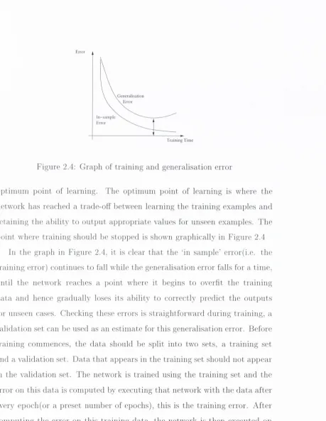
oi)tiniuni i)oint of learning. T he o p tim u m point of learning is where th e network has reached a trade-off between learning the tra in in g exam ples and re ta in in g th e ability to o u tp u t aj)propriate values for unseen examples. T h e jjoint where tra in in g should be sto])ped is shown graphically in Figure 2.4

mini-inuiii the network should be saved as the point of niaxirnuin generalisation.

Once this error rises for a preset number of e])ochs or the training reaches

a preset maxinnim number of epochs, training should be stopped and the

saved network should be returned as the “best” network.

2.2.2

B ia s & V ariance in N eu ral N etw ork s

Tlie final consideration when training neural networks is to balance the errors

due to bias and variance. These two errors are not independent, reducing one

will cause an increase in the other. In short, a network fitting the training

d a ta closely will have a low bias but a higher variance, while a netw^ork with

a low'er variance will lead to a decrease in the fit of the training data. For

optimal learning it is necessary to l)alance both of these factors.

The bias/variance dilemma was studied in some detail by Geman et al.

[30]. In this paper, the authors show in detail the bias/variance decomposi­

tion of mean-S(iuared error. This is of particular interest for backproi)agation

nc'ural networks as this is the most used error function for these networks.

E(iuation 2.1 shows the breakdown derived by Genian et al. for the mean

scjuared error.

( / ( x ; P ) - i ? p [ / ( x ; P ) ] ) 2

The bias and variance of this ecjuation are averaged over the possible

training sets

V .

The function / ( x ; P ) is the prediction of the network on an

example x given the network trained on the set

T>.

The desired response is

to the regression

E[y\x\.

This vahie is then averaged for the set of possible

training sets

V.

On the right the first part of this equation measures the bias. The bias

can be thought of as the average distance of a network function / trained

on a set of d a ta

V

from the true regression for the same inj^ut x. If on

average there is a big difference, the bias is said to be large. In general, this

will depend on the probability distribution

P

of the d a ta and how

T>

reflects

this distribution. The same network may be biased in some cases but not in

others.

The second part of this equation on the right hand side measures the

variance. This measures the average distance of a network / trained on a set

of d a ta

D

from the average distance of other networks trained on different

sets of data.

\ ariance for a single network can be controlh'd by combining examples

th a t are nearby in the in])ut si)ace. However, this will ty])ically increase

the bias of th a t network, as details of the regression are lost, e.g. peaks and

valleys art' blurred. Bias for a single network can be controlled by introducing

more hidden units into the network. This has the effect of increasing the

complexity of the function th a t the neural network can learn. It is, however,

likely to increase the variance significantly.

Therefore, to achieve a low error, it is necessary to reduce both the bias

and the variance components. Typically, reducing one of these will cause an

incr('ase in the other. This is commonly known as the l)ias/variance trade-off.

C hapter 3

E nsem bles

R e c e n t rese a rc h in m a c h in e le a rn in g a n d , in p a r t i c u l a r , n e u r a l n e tw o rk s h a s

b e g u n t o ex])loit t h e pow er o f t r a i n i n g m u ltip le le a rn e rs t o a p p r o x i m a t e t h e s a m e f u n c tio n . T h e s e n u iltip le learners, collectively k now n as a n ensemble, w ere first i n tr o d u c e d l)y H a n s e n & S a la m o n [32], B y c o m b in in g th e p r e d ic ­ tio n s fro m th e s e learners, it is possible to increase th e a c c u r a c y of t h e p r e ­

d ic tio n s a n d in t h e process re d u c e th e i n s t a b ility of p re d ic tio n s . I n s t a b il it y ref('rs to t h e p h e n o m e n o n w h e re b y two n e u ra l n e tw o rk s t r a i n e d t o a p p r o x ­ i m a t e t h e s a m e fu n c tio n m a y a c tu a ll y o u t p u t very different re s u lts for n e w e x a m p le s , de])e n d in g on th e in itia l c o n d itio n s a n d t h e t r a i n i n g j) a r a m e te r s

used.

I t is i n te r e s t in g to n o te t h a t a lt h o u g h t h e id e a of c o m b in in g m u lt ip l e m ac liin e le a rn e rs is re la tiv e ly recent, th e in cre ase d a c c u r a c y o b t a i n a b l e fro m

a c o m m i t t e e o f e x p e r t s is not. As long ago as 1784, th e M a rq u is of C o n d o r c e t ])ut fo rw a r d th e t h e o r e m , now know n as th e C o n d o r c e t J u r y T h e o r e m [18]:

“I f each v ot er has a proba,hi,lif4j p of being correct and the proba.bility of a,

ma'jority of v ote rs being correct is M , then p > 0.5 impl ies M > p. In the

l imi t M approaches 1, f o r all p > 0.5 as the number of voters approach,es

A m ore accessil:ile mocierii reference for this theorem is N itzan an d P a ro n sh [44]. T h e first p a r t of this theorem is not controversial, it is easy to show t h a t if a new com m ittee m em ber makes correct decisions more t h a n half of the tim e and makes different mistakes to th e rest of th e c o m m ittee th e n th e perform ance of the com m ittee will im prove w ith the addition of tliis new m em ber. However, in practice the second claim is unlikely to be true. A very large com m ittee will not, in practice, be right all of the time. It will n ot be j)ossible to find new mem bers t h a t will increase th e diversity of the connnittee; instead their voting behaviour will be collinear w ith some exist­ ing m em bers of th e conunittee. Ty])ically th e diversity of th e ensemble will p la te a u as will the accuracy of the ensenil)le a t some size between 10 and 50 m embers.

In order to get the l)est possible results from an ensemble, it is preferable t h a t a large degree of diversity exists am ong th e m em bers of t h a t enseml)le. T h a t is, th e m em bers should all be experts in localised areas of th e in p u t sijace. T h e reason for this is (juite simple. If all of the m em bers either predict the sam e answers or are all (^xperts in roughly the sam e area of th e in p u t space, th e n the existence of more th a n one such learner does not supply any m ore inform ation th a n a single network alone. M ethods of in tro d u cin g diversity into these learners are outlined in section 3.1.

T h ere are several m e thods available for com bining th e results. A few of these have been chosen and are outlined in section 3.2.

3.1

Training M u ltip le D iverse Learners

sense to think of this trade-off in terms of the error/am biguity model de­

scribed first by Krogh &: Vedelsby [37].

Krogh & Vedelsby’s foriinila for describing the error/am biguity of an en­

semble is derived in full by Zenobi [67]. In their decomposition they ex]:)ress

the bias and variance components of the ensemble error as the weighted en­

semble error and the ensemble ambiguity (diversity). Their equation relating

these variables is given in Equation (3.1) where

E

is the ensemble error,

E

is the weighted ensemble error and

A

is the w'eighted ambiguity measure.

E = E - A

(3.1)

Instead of expressing the averages for error and ambiguity over different

training sets, Krogh & Vedelsby use the weighted averages over the ensemble.

If th(' enseml)le is strongly biased the ambiguity will be small, because the

networks implement very similar functions and thus agree on inputs even

outside the training set. A larger variance betw'een the networks will make

the ambiguity higher and in this case the generalisation error will be smaller

than the average generalisation error.

There are several methods connnonly used to introduce this ambiguity

into ensembles. All of these methods work to some degree by skewing the

number or type of examjiles being presented to the individual networks during

training. The methods j)resented below include:

•

Section 3.1.1 - Bagging

•

Section 3.1.2 - Boosting

•

Section 3.1.3 - Cross validation

By skewing th e distrib u tio n of exam ples being presented to each of th e networks using one of these m ethods, the networks tra in in g should be con­ c e n tra te d on different exam ples to other networks in th e ensemble. In th is

way, th e am biguity can l)e increased between networks as they will m ake

m istakes in different areas of the in p u t space. This is equivalent to ad d in g m ore m e m bers to the M arquis de C o n d o rc e t’s com m ittee who have differ­

ent opinions and hence make different mistakes thus increasing th e overall i:>redictive accuracy of the com m ittee.

3.1.1

B a g g in g

Bagging, sho rt for “b o o ts tra p aggregating” , was introduced by Breinian [10]. T h e first p a r t of bagging is th e process of t)00ts tra p p in g the in p u t examples.

B ootstra i)ping is a pop u la r statistical technique of sam pling a d a ta s e t w ith replacem ent [10], W hen sam pling N tim es from a d a ta s e t of size N, a p p ro x ­ im ately 63% of the exam ples will be chosen a t least once. T his set of d a t a is then used as the tra in in g d a t a for the chosen machine learning prediction algorithm . In the case of neural networks, th e rem aining d a t a can be used to prevent o verhtting d uring training. In bagging, Breinian suggests using

an average as the m e th o d for com bining the results. Averaging is covered in more detail in section 3.2.1.

3 .1 .2

B o o s t i n g

T h e original work on boosting was performed by Schapire [51]. T h e basic

idea b ehind this work is to build a weak learner using th e available d a t a and using an equal i)robability for the selection of each exam ple in th e d a ta . Once

this learner has been built the probabilities of th e exam ples in th e d a ta s e t

O ne of the m ost pop u la r im plem entations of this m e th o d is t h a t used by

F reund & Schapire [26]. This is outlined in detail below:

T h e initial weights of each exam ple in th e train in g are set as uniform, i.e.

Di {t ) = jf, where N is the to ta l n u m ber or train in g examples. T h e objective

now is to minimise the weighted error:

Cf, = / g,) (3.2)

i

where / is th e indicator function, lit is the current hypothesis and (ji is the

tru e goal class.

If ^ 2’ o u tp u t w ith T = t — 1.

O therw ise set:

n^ = log ---- ^ (3.3)

and finally u p d a te the distribution of weights on th e tra in in g set:

A + i ( '0 = A ( * ) e (3.4)

where Z/ is a norm alisation factor (chosen so t h a t A + i is distrib u tio n ).

T h e final o u tp u t classifier H { x ) is:

I I ( x ) = (ITg n m x f { x , g) = a r g m a x ( > n t l { h t { x ) = g )) (3.5)

qec ' ' ' V ^ ^ ' /

t=l

Diversity is thus built into the models d u rin g construction by virtue of

th e fact t h a t each model focuses its train in g on different examples.

B oosting does raise an overfitting problem. P a rticu larly noisy d a t a could

tra in some of the models on b ad d ata. These models would provide very

ensemble. The i)ioblem of overfittiiig using boosting and in i)articular the

AdaBoost method is raised in MacUn & Opitz [39].

3.1 .3

C ross V alid ation E n sem b les

K-fold cross validation relies on sj^litting the available data,

D,

for training

into a total of

K

sets,

Di, D

, . . . ,

D^.

This approach is used by Krogh &

Vedelsby in their paj^er analysing the bias and variance components of neural

networks in terms of error and ambiguity [37].

A total of

K

networks are then trained on these sets, each time using all

but one of the sets(D

D^)

as training d a ta and using the remaining

set(Dk)

for testing the generalisation error of the network during training and thus

overhtting.

K-fold validation makes good use of the available d a ta and introduces

reasonable diversity as long as all of the sets are a fair rei)resentation of the

d a ta distribution.

3 .1 .4

F eature S u b sets

A rc'cent method used to introduce diversity into ensemble members involves

training each member using a different feature mask [68]. Each mask is a

boolean string with a length ecjual to the number of features in the training

data. In this string I ’s correspond to features th a t should l)e used in the

training of a network and O’s correspond to features th a t should be omitted.

The masks axe produced using a wrapper method. The wrapper method

a])proach involves estimating the “goodness” of each mask with respect to

the bias of the individual network type. A summary of the mask production

algorithm as described in [21] is shown below:

cross v a lid a tio n .

2. S t a r t i t e r a t i n g t h r o u g h th e m a s k

3. F lip th e c u r r e n t b it o f th e m a s k a n d e s t i m a t e t h e g e n e r a li s a ti o n e rr o r

of t h e new m a s k using cross v a lid a tio n

4. If t h e new m a s k h a s a lower e rr o r t h a n t h e p re v io u s m a s k , t h e n a c c e p t

th is bit Hi]), o th e rw is e reverse t h e flip a n d r e t a in t h e o r ig in a l m a s k

5. Tf t h e e n d of th e m a s k h a s n o t be e n r e a c h e d t h e n c o n tin u e f ro m Stej) 3

C. If no b it Hips have be e n a c c e p te d t h e n o u t p u t t h e c u r r e n t m a s k as

oi^tinuun, o th e rw is e c o n tin u e from S te p 2

A m o re conij)lex v a ria tio n on th is a l g o r i th m is d e s c rib e d by Z e n o b i [68].

In th is v a ria tio n , Zenobi d e scrib es how f e a tu r e s u b s e ts c an b e f o u n d t h a t

m a x im is e t h e t o t a l a m l)iguity in t h e ensem ble.

T h e a l t e r n a t i v e to th e w r a p p e r a p p r o a c h d e s c r ib e d al)Ove is t o s im p ly

use r a n d o m m ask s. R a n d o m m a s k s do h elp to i n tr o d u c e diversity, b u t a t t h e

cost of h ig h e r erro r. A g o o d w ra p i)e r techniciue s h o u ld on a v e ra g e o u t])e rfo rm

r a n d o m m asks.

3.2

C om bining resu lts

O n c e a n ensernl)Ie of n e tw o rk s is t r a i n e d , th e r e s u lts from each netAvork m u s t

1 ) 0 c o m b in e d so as to p re s e n t a single r e s u lt to th e user.

For cla ssifica tion task s, th e s im p le s t m e t h o d is to s im p ly v o te a m o n g th e

netw o rk s, w it h t h e m a j o r i t y c;lass d e c la re d as t h e j^redicted class.

T h e i)roblem is s o m e w h a t m o re difficult for regression task s. T h e r e a re a

strengths. T h ree of these niethocis, averaging, linear regression and principal

co m ponents regression are detailed below. A brief description of th e ])roblems

solved by these m e thods is included for clarity.

3 .2,1

A v e r a g in g

A veraging results is th e m e th o d used by Breirnan in his p a p e r on bagging [10].

Perrone & C ooper [45] also make reference to this techni(}ue which th e y call

the Basic Ensem ble M eth o d ( “B E M ” ). A veraging works by assigning equal

w eights(l/iV , where N is the to tal n um ber of networks in th e enseml)le) to

the predictions of each neural network in the ensemble.

1

1 = 0

3 .2 .2

L in ear R e g r e s s io n

Linear regression has been independently studied by several researchers, [45,

33].

P errone <k C ooper refer to their m e th o d as th e Generalised E nsem ble

M e th o d (G E M ). In this m ethod they minimise the m ean sfjuared error in

order to set th e weights, ai, w ith respect to the ta rg e t function f { x ) . T h e

form ula they suggest for calculating these weights is shown in Eciuation 3.7.

rv, = (3.7)

Ylk '^ j ^kj

T h e m i { x ) above are defined as th e difference between th e tru e value of

th e function and th e value predicted l)y network i, i.e. f { x ) — f i { x ) .

ft is im p o r ta n t to note t h a t the columns in the Ci j m a tr ix should be

uncorrelated. Correlation between columns will lead to th e m a trix being

u n stab le when inverted. To avoid this problem th e y suggest d ro p p in g all b u t

one of any correlated grouj) of columns. T his should not result in a great

loss of accuracy. T h e ]:)robleni of correlated columns is dealt w ith again in

Section 3.2.3.

T h e weights produced by Perrone & C ooper will be s u b ject to th e con­

s tr a in t = 1- lu the more general case of linear regression, this

c o n strain t is n ot applical)le.

3 .2 .3

P r in c ip a l C o m p o n e n t s R e g r e s s io n

Principal C o m p o n e n ts R egression(“P C R * ” ), was developed by Merz & Paz-

zani [40], P C R * was developed w ith the goal of elim inating the j^roblem

of colliuearity of networks while still predicting weights t h a t j)rovide a high

levc'l of accuracy. Collinearity can lead to very unstab le m atrices when in­

verting m atrices, an unavoidable step when using any linear regression i)ased

m ethod.

Merz & P azzani identify three m e th o d s for reducing th e problem of collinear­

ity. T h ey are;

• T rain models to have uncorrelated errors by a d ju stin g th e bias of th e

learning algorithm .

• Use a gradient descent technique for s ettin g th e weights.

• Use a linear regression m e th o d w ith constraints on th e possible weights

None of these sohitions provide a full answer to the problem. Models

naturally have a certain level of collinearity so even explicit training may not

always eliminate this collinearity. Gradient descent techniques are j^rone to

getting stuck in local minima and not finding optimal solutions. Finally, con­

strained linear regression may also lead to sub optimal weighting solutions.

The basic algorithm of PCR* is set out below:

InjMit: A^, the m atrix of predictions of the models in

F

1. C =

cov{k^'')

2. P C =

PC A[ C)

3.

K

= Choose_Cutoff(PC)

4.

= /^iP C , + . . . +

/ 3 j , P C ,

= ( P C ] , P C a - ) - V

6. Returncv

In the above algorithm, C is the covariance m atrix for the predictions .4^'

and P C is the set of princii)al components based on the m atrix C.

The search aspect of PCR* is in step 3, where the mirnber of j)rincipal

components th a t are going to be used in the determination of the weights

is found. The authors of PCR* show how cross validation is one techniciue

tliat may be used to judge the error on different subsets of the princij)al

components. The optimal number of components to use is taken at the point

of mininnim error.

In Step 4, linear least squares regression is used to derive an estimate of

coinljining future predictions from the ensemble of networks by expanding

the equation in Stej) 4 to

PC^

7

the weights to be the coefhcients of the original n etw o rk s(/j).

A lthough Merz & P azzani developed P C R * to use all of th e networks,

s ta tin g t h a t “correlation could be handled w ith o u t elim inating any of th e

learned m odels” , it is only fair to refer to oth e r work in th e area of elim inating

correlation. One such j)iece of work has been done by Zhou [70] in which he

does d rop models in order to reduce th e correlation and hence instability in

assigning weights to ensemble members.

3.3

S u m m a r y

T h e ensembles used in the E valuation chapter of this thesis were built us­

ing bagging to o b ta in m axim um diversity. Bagging is a flexible m e th o d for

building enseml)les providing good, stable perform ance over a wide variety of

d atasets. It makes good use of all of the d a t a in building th e enseml)le and

avoids problem s of learning noise in the d a ta s e t som etim es associated w ith

])oosting.

T he d a ta s e ts evaluated were b o th classification j)roblems and hence a

C hapter 4

R u le Learning A lgorithm s

Rules are arguably one of the simplest representations of knowledge in a

m achine learning system. T h eir simple, directly in terp reta b le form has w'on

th e m a strong following th ro u g h o u t the machine learning fraternity. Decision

trees represent a si)ecialised set of rules organised in branches and leaves.

W'hen followed in an order determ ined by an exami)le case, th e branches will

lead to a single leaf node. This node will have a class associated witli it and

this is used as th e prediction o u tp u t. Decision trees are readilj^ decom posable

to i)ro])ositional rule sets.

Each rule is typically w ritten in the form of an IF clause which contains

one or more term s, the conditions of which m ust be m et in order to “fire”

t h a t rule. W h e n a rule is fired, the class associated w ith th e rule, usually

w ritte n as a T H E N clause is either counted as a vote tow ard an overall class

p rediction or it is presented directly to the user as th e predicted class. An

exam])le rule is shown below:

IF Sa_02_2 > 91.89

AND Dehydration=None

AND Retractions=0

THEN DISCHARGE

Rules such as in the exam ple above, m ay be generated by a variety of m ethods. Rule extra ction from neural networks is covered in C h a p te r 5. An in tro d u c tio n to decision trees is covered in section 4.1 and rule ex tra c tio n from these is covered in section 4.1.3. A lgorithm s for g enerating rules directly are covered in section 4.2, these include CN2, F O IL and FOCL.

Tom M itchell’s book Machine Learning [43] is an excellent general in tro ­ d u ctio n to the areas of decision trees and rules.

4.1

D e c isio n T rees

Decision trees comprise a very po p u la r set of machine learning m ethods. T h e ir poj^ularity is due to their proven accuracy in m odelling a wide range of problem s [58, 53]. In addition to th eir good perform ance, th e y are easily iu t('rpretable by experts involved in the field of study.

Decision trees o perate l)y p a rtitio n in g in p u t features on axis-parallel b o u n d ­ aries; each such p artitio n is known as a decision node. Each decision node m ay have one or more child nodes. T he child node(s) m ay be either a decision node or a leaf node. Leaf nodes have a class associated w ith th e m and can n ot have any children. Once a leaf node has been reached when processing a decision tree, processing stops and the class associated w ith t h a t child is re tu rn e d as a prediction to th e user.

P e t a l Length <= 1. 9 ; I r i s - s e t o s a ( 5 0. 0 )

P e t a l Length > 1 . 9 :

I

P e t a l Width > 1 . 7 : I r i s - v i r g i n i c a ( 4 6 . 0 / 1 . 0 )

I

P e t a l Width <= 1.7 :

I

I

P e t a l Length > 5 . 3 : I r i s - v i r g i n i c a

( 2 . 0 )

I

I

P e t a l Length < = 5 . 3 :

i

I

I

P e t a l Length < = 4 . 9 : I r i s - v e r s i c o l o r ( 4 8 . 0 / 1 . 0 )

I

I

I

P e t a l Length > 4 . 9 :

I

I

I

I

P e t a l Width <= 1 . 5

: I r i s - v i r g i n i c a ( 2 . 0 )

I

I

I

I

P e t a l Width > 1 . 5

:

I r i s - v e r s i c o l o r ( 2 . 0 )

F igure 4.1: E xam ple decision tree using Iris d a t a

O ne m a jo r disadvantage of trees is in the way t h a t they can only p a rtitio n

features on axis parallel boundaries. If a class is n a tu ra lly p a rtitio n e d by a

hyperi)lane t h a t does not lie parallel to axis boundaries, then m any decision

nodes on several features may l)e required to accurately re])resent this deci­

sion boundary. This problem can be seen in Figure 4.2. In this figure, the

splits nuide by th e decision tree are represented by th e broken line. A neural

network would have little troul)le finding a co m pact solution to this problem ,

however, a h u m a n user of a system would have great troul)le visualising th e

m a th e m a tic a l solution presented by the network.

4 .1 .1

C 4 .5

O ne of the m ost po p u la r algorithm s used for building decision trees is Q u in ­

l a n ’s C4.5. T h e p o p u la rity of this program stem s from its freely available

im p le m e n ta tio n (with accom panying source code) and its proven perform ance

ov(!r a wide variety of domains.

B u ild in g a T ree

B uilding a tree in C4.5 involves searching each of the features to find th e one

Figure 4.2; D ata th a t is ill suited for decision tree learning.

split of a feature is crucial. If the most discriminating features are chosen

at each stage in building a decision tree, the tree will tend to i)e small.

A small tree represents a concise concei)t description for the hypothesis,

thus satisfying Occams razor (i.e. where tw'O or more descriptions exist, the

simplest of these should l)e i)referr('d).

To understand the C4.5 measure of information, it is useful to look at

ID3, an algorithm for building decision trees also i)roi)Osed by Quinlan [46].

In this algorithm, Quinlan used a gain criterion to assess the information

content of s])littiug a set of data. Quinlan himself sums up this criterion

with the statement: “The information conveyed by a message depends on its

probability and can be measured in bits as minus the logarithm to base 2 of

th a t ])robability.”

The probability of selecting a class,

Cj

from a set

S

is

freq{Cj, S)

|

5

- l o g , hits (4.2)

To find the expected inform ation for a message w ith a class Cj w ith res])ect to class membershij), sum over all the classes in p ro p o rtio n to th eir frequencies in S:

r n f o i S ) = - ± X log,