Combined Genetic Algorithm Optimization and Regularized Orthogonal
Least Squares Learning for Radial Basis Function Networks
S. Chen,
Senior Member, IEEE, Y. Wu, and B. L. Luk
Abstract—The paper presents a two-level learning method for
radial basis function (RBF) networks. A regularized orthogonal least squares (ROLS) algorithm is employed at the lower level to construct RBF networks while the two key learning parameters, the regularization parameter and the RBF width, are optimized using a genetic algorithm (GA) at the upper level. Nonlinear time series modeling and prediction is used as an example to demonstrate the effectiveness of this hierarchical learning approach.
Index Terms— Genetic algorithms, orthogonal least squares
algorithm, radial basis function networks, regularization.
I. INTRODUCTION
T
HE GA [1], [2], as a powerful nonlinear optimization technique, has been used to learn neural-network topolo-gies as well as the weights in fixed network structures (e.g., [3]–[7]). A key advantage of using the GA as a neural-network learning method is that it is capable of achieving optimal or near-optimal network topology and weight settings under given training conditions. This is, however, obtained at the cost of extensive computational requirements. In particular, direct optimizing the network weights using GA’s is hampered by difficulties of high evaluation cost and slow convergence.Simpler learning can often be achieved if a neural network has a linear-in-the-parameters structure. When the width pa-rameter is fixed and a set of RBF centers is provided, a RBF network has such a structure and an orthogonal least squares (OLS) algorithm [8] has been developed for constructing parsimonious RBF networks. Other construction algorithms based on the parsimonious principle have been derived for “linear-in-the-parameters” neural networks (e.g., [9]–[11]). A well-constructed small neural network often has desired generalization properties.
If training data are highly noisy, the parsimonious principle alone may not be sufficient to guarantee good generalization performance. Regularization is one of the principal techniques for improving the generalization properties [12]–[14]. By combining the parsimonious principle with a regularization method, a ROLS algorithm [15] has been derived for con-structing RBF networks under severely noisy conditions. A good regularization parameter required by the ROLS algorithm is usually obtained by iterations using a Bayesian formula [13].
Manuscript received December 23, 1998; revised May 25, 1999. S. Chen is with the Department of Electrics and Computer Science, University of Southampton, Highfield, Southampton SO17 1BJ, U.K.
Y. Wu is with the Department of Radiation Oncology, William Beaumont Hospital, Royal Oak, MI 48073 USA.
B. L. Luk is with the Department of Electrical and Electronic Engineering, University of Portsmouth, Anglesea Building, Portsmouth PO1 3DJ, U.K.
Publisher Item Identifier S 1045-9227(99)07236-7.
The regularization parameter so generated, however, may not necessarily be the best one since the regularization parameter is strongly coupled with some other learning parameter, as will be demonstrated later.
We propose a two-level learning hierarchy for construct-ing RBF networks based on the combined GA and ROLS algorithms. Because the generalization performance is a com-plex multimodal function on the space of the width and regularization parameters, these two parameters are optimized using the GA at the upper level. Given these two parameters, the ROLS algorithm is used to construct parsimonious RBF networks at the lower level. Since the GA only optimizes two parameters and the lower layer only involves linear learning problems, the computational complexity of this combined approach is much less than that of using the GA to learn all the network parameters directly. RBF networks produced by this learning hierarchy have superior generalization performance as is demonstrated by the included examples of nonlinear time series modeling.
II. THE ROLS ALGORITHM
The RBF network considered in this paper has a single output and a Gaussian nonlinearity with a uniform width . Specifically, the network output is defined by
(1)
where is the network input vector, is the number of nodes, are the weights, are the center vectors and denotes the Euclidean norm. Although each node may have a different width and for some applications adjusting individual widths can often improve performance [16], a uniform width is sufficient for the RBF network to achieve universal ap-proximation [17]. Using a uniform width obviously results in a simpler learning process. Replacing the Euclidean distance in the standard RBF network by the Mahalanobis distance gives rise to a more general neural-network model [16], [18]. A novel Gaussian-bar network has also been proposed [19]. We will concentrate on the simple network model (1). The approach developed, however, is not restricted to this particular Gaussian RBF network and can readily be applied to multioutput RBF networks [20].
Assume that a training set of samples
is available, where is the desired network output cor-responding to the network input . In order to obtain a “linear” regression model, each is considered as a
candidate center, that is, for , and a
1240 IEEE TRANSACTIONS ON NEURAL NETWORKS, VOL. 10, NO. 5, SEPTEMBER 1999 fixed width is given. By defining
(2)
we can express the desired output as
(3)
where is the error between and the actual network output . By introducing
(4)
(5)
(6)
(7)
(8)
we can rewrite the system (3) in the matrix form
(9)
The ROLS algorithm is an efficient forward subset selection procedure for constructing a smaller subset model from the full regression model (9).
Let an orthogonal decomposition of the regression matrix
be , where satisfies
for , and is an upper triangular matrix with unit diagonal elements. The system (9) can be rewritten as
(10)
where
(11)
is the orthogonal weight vector. The ROLS algorithm selects a subset of significant regressors based on the following regularized error criterion:
(12)
where is a regularization parameter. The detailed selection procedure can be found in [15] and will not be repeated here.
In this “linear” learning approach, the width parameter is fixed to some constant. Obviously, it is desirable to adjust the width during learning. However, nonlinear learning methods would be required since the network output is strongly nonlin-ear with respect to . The ROLS algorithm adopts the evidence procedure [13] to estimate a regularization parameter. Given an initial guess of , the algorithm constructs a subset model. This in turn allows an updating of using the formula
(13)
where
(14)
[image:2.612.339.520.64.170.2]is the number of good parameter measurements [13] and is the size of the subset model. After a few iterations, an
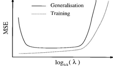
Fig. 1. Usually assumed characteristics of mean square error as a function of regularization parameter. Notice that this generalization curve is not generally correct.
appropriate value can usually be found. The regularization parameter so determined, however, may not be an optimal one, as will be shown later.
III. THECOMBINED GAANDROLS LEARNING
To understand the motivations of using a global optimization method to learn the regularization parameter and width, it is best to examine the generalization performance as a function of these two parameters. It is often observed that regularized learning exhibits the characteristics of Fig. 1 [12], [15]. This appears to suggest that generalization performance curves may have a single low flat region, and a gradient algorithm such as the iterative evidence procedure of (13) will be able to lead to a good in this region. It should be emphasized that the evidence procedure in general can only obtain a local optimal value of and Fig. 1 does not provide a complete picture. In fact, the generalization performance is a highly complicated multimodal function on the space of and . The characteristics of Fig. 1 may only be obtained under a particular value of .
We use a simple example to demonstrate these points. Consider the modeling of the scalar function
(15)
by a Gaussian RBF network. The training data was generated from , where the Gaussian noise had a zero mean and variance 0.02 and was taken from the uniform distribution in . The training data had a signal-to-noise ratio (SNR) of 14 dB. Given values of and , the ROLS algorithm constructed RBF networks. The learning procedure was terminated when the regularized error reduction ratio [15] was smaller than a preset threshold. RBF models constructed had five to seven nodes depending on the values of and . The generalization performance, the mean square error (MSE) between the noise-free system output and the network response , was computed. The inverse of this MSE as the function of and is depicted in Fig. 2.
Fig. 2. Surface of the inverse generalization performance on the space of and .
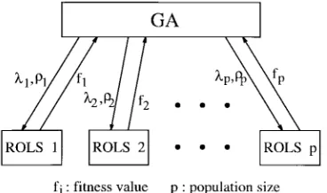
Fig. 3. Schematic of two-level learning hierarchy for RBF networks.
as illustrated in Fig. 3. At the upper level, the GA, with a population size of , learns the width and the regularization parameter based on the fitness function values provided by the lower level. The lower level consists of the parallel ROLS algorithms, one for each pair of and provided by the GA. The data set is divided into a training set and a validation set. The th ROLS algorithm constructs a RBF network using the training data set with given and . The generalization performance, the MSE over the validation data set, of the resulting RBF model is computed. The inverse of this generalization performance is the fitness function value for the given and .
With the goal being to find a global optimum solution as quickly as possible, we adopt the so-called micro-GA [21]. This version of GA uses a population that is much smaller than typically employed. In the original work [21], it was reported that the micro-GA can find optimal regions faster than standard GA’s for selected optimization problems. However, allowing a single sequence of a micro-GA to converge may not be very useful apart from quickly locating local optima. Therefore, af-ter such convergence, the population is reinitialized randomly while the best individual found up to that point is copied into the newly generated population. This iterative reinitialization is repeated until no further improvement is evidenced. The two parameters, and , are each coded into a 16-bit string, and a population size of is used. The crossover rate is set to 1.0, with the number of crossover points typically set to four.
No mutation is employed, as the reinitialization routine serves to introduce diversity. Tournament selection [21] is employed to determine parents for reproduction.
The computational complexity of the proposed two-level learning scheme is determined by the total number of function evaluations at the upper level. Assume that the micro-GA con-verges after generations and the complexity of the ROLS algorithm is . Then the complexity of the combining GA and ROLS learning scheme is
(16)
Since the micro-GA is only used to optimize the two key parameters and the lower level involves linear learning prob-lems, the overall computational requirement of the proposed scheme is well within the computing power of a standard PC. The micro-GA employed is specifically designed to minimize the required number of function evaluations at the upper level. In contrast, using a GA directly to determine the network structure as well as to learn all the network parameters [5]–[7] will require far more extensive computation.
IV. NONLINARTIME SERIES APPLICATION
Nonlinear time series modeling and prediction are used to illustrate the combined GA and the ROLS learning approach.
A. Example 1
[image:3.612.78.262.285.394.2]1242 IEEE TRANSACTIONS ON NEURAL NETWORKS, VOL. 10, NO. 5, SEPTEMBER 1999
[image:4.612.343.520.62.180.2]Fig. 4. Generalization performance with and without regularization for ex-ample 1.
Fig. 5. Convergence behavior of the GA for example 1 with a SNR of 14 dB.
Fig. 4 depicts the generalization performance, the MSE between the noise-free system output and the actual RBF model output , for these two cases. It can be seen that the simple regularization technique employed has superior generalization performance under highly noisy training condi-tions. For the training data of SNR = 14 dB, it was observed that the optimal regularization parameter
and width , corresponding to the highest peak in Fig. 2, was achieved by the combined GA and ROLS learning. To examine the convergence behavior of the GA, Fig. 5 plots the best fitness value versus the number of fitness function evaluations with a SNR of 14 dB.
B. Example 2
The second example was Mackey–Glass time series predic-tion. The data was generated using the following equation:
(17)
where and initial conditions for
. A sampling step size of 2 s was used, and Gaussian white noise was added to the time series samples, giving rise to a SNR of 40 dB. A data set of 1000 noisy samples were obtained with the first 500 samples used as the training set and the last 500 samples as the validation set. The input vector to the Gaussian RBF predictor at was . The RBF predictors were constructed with and without regularization. Again in the case of no regularization, the upper level only learned . The RBF predictor constructed with regularization had 18 centers while the predictor obtained without regularization had 24 centers. The multistep prediction accuracies over the validation set
[image:4.612.351.513.220.322.2]Fig. 6. Multistep prediction performance for Mackey–Glass time series.
Fig. 7. Multistep prediction performance for sunspot time series.
were then computed and the results are plotted in Fig. 6. From Fig. 6, it can be seen that better generalization performance was achieved with regularization when the prediction step is large.
C. Example 3
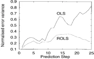
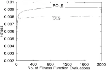
This example was sunspot time series prediction based on the 280 sunspot observations over the years 1700 to 1979. The observations of 1752 to 1979 were used as the training set and the observations of 1700 to 1767 were used as the validation set. Two Gaussian RBF models of 25 centers were constructed using the two-level learning hierarchy with and without regularization. The model input vector consisted of eight past observations. The normalized multistep prediction accuracies of the two resulting models over the validation set are plotted in Fig. 7, where it can be seen that the combined GA and ROLS learning has superior generalization performance. The convergence speeds of the two-level learning hierarchy with and without regularization are illustrated in Fig. 8.
V. CONCLUSIONS
[image:4.612.89.251.226.328.2]effi-Fig. 8. Convergence behavior of the GA for sunspot time series modeling.
cient compared with using the GA directly to construct the network model. Time series modeling and prediction have been used to demonstrate superior generalization properties of the combined GA and ROLS learning approach.
REFERENCES
[1] J. H. Holland, Adaptation in Natural and Artificial Systems. Ann Arbor, MI: Univ. Michigan Press, 1975.
[2] D. E. Goldberg, Genetic Algorithms in Search, Optimization, and
Ma-chine Learning. Reading, MA: Addison-Wesley, 1989.
[3] D. J. Montana and L. Davis, “Training feedforward neural networks using genetic algorithms,” in Proc. 11th Int. Joint Conf. Artificial Intell., San Mateo, CA, 1989, pp. 762–767.
[4] L. Yao and W. A. Sethares, “Nonlinear parameter estimation via the genetic algorithm,” IEEE Trans. Signal Processing, vol. 42, pp. 927–935, 1994.
[5] V. Maniezzo, “Genetic evolution of the topology and weight distribution of neural networks,” IEEE Trans. Neural Networks, vol. 5, pp. 39–53, 1994.
[6] P. J. Angeline, G. M. Saunders, and J. B. Pollack, “An evolutionary algorithm that constructs recurrent neural networks,” IEEE Trans. Neural
Networks, vol. 5, pp. 54–65, 1994.
[7] S. A. Billings and G. L. Zheng, “Radial basis function network config-uration using genetic algorithms,” Neural Networks, vol. 8, no. 6, pp. 877–890, 1995.
[8] S. Chen, C. F. N. Cowan, and P. M. Grant, “Orthogonal least squares learning algorithm for radial basis function networks,” IEEE Trans.
Neural Networks, vol. 2, pp. 302–309, 1991.
[9] M. Brown and C. J. Harris, Neurofuzzy Adaptive Modeling and Control. Englewood Cliffs, NJ: Prentice-Hall, 1994.
[10] T. Kavli, “ASMOD: An algorithm for adaptive spline modeling of observation data,” Int. J. Contr., vol. 58, no. 4, pp. 947–968, 1993. [11] L. X. Wang and J. M. Mendel, “Fuzzy basis functions, universal
approximation, and orthogonal least-squares learning,” IEEE Trans.
Neural Networks, vol. 3, pp. 807–814, 1992.
[12] C. Bishop, “Improving the generalization properties of radial basis function neural networks,” Neural Comput., vol. 3, no. 4, pp. 579–588, 1991.
[13] D. J. C. MacKay, “Bayesian interpolation,” Neural Comput., vol. 4, no. 3, pp. 415–447, 1992.
[14] F. Girosi, M. Jones, and T. Poggio, “Regularization theory and neural-network architectures,” Neural Comput., vol. 7, pp. 219–269, 1995. [15] S. Chen, E. S. Chng, and K. Alkadhimi, “Regularised orthogonal least
squares algorithm for constructing radial basis function networks,” Int.
J. Contr., vol. 64, no. 5, pp. 829–837, 1996.
[16] M. T. Musavi, W. Ahmed, K. H. Chan, K. B. Faris, and D. M. Hummels, “On the training of radial basis function classifiers,” Neural Networks, vol. 5, no. 4, pp. 595–603, 1992.
[17] J. Park and I. W. Sandberg, “Universal approximation using radial-basis-function networks,” Neural Comput., vol. 3, pp. 246–257, 1991. [18] S. Lee and R. M. Kil, “A Gaussian potential function network with
hierarchically self-organizing learning,” Neural Networks, vol. 4, pp. 207–224, 1991.
[19] E. J. Hartman and J. D. Keeler, “Predicting the future: Advantages of semilocal units,” Neural Comput., vol. 3, no. 4, pp. 566–578, 1991. [20] S. Chen, P. M. Grant, and C. F. N. Cowan, “Orthogonal least squares
algorithm for training multioutput radial basis function networks,” in
Proc. Inst. Elect. Eng., vol. 139, pt. F, no. 6, pp. 378–384,1992.
[image:5.612.78.263.62.183.2]