Trajectory Tracking Controller Design for A Tricycle Robot Using Piecewise Multi-Linear Models

(1)

Trajectory Tracking Controller Design for A

Tricycle Robot Using Piecewise Multi-Linear

Models

Tadanari Taniguchi and Michio Sugeno

Abstract—This paper deals a tracking trajectory controller design of a tricycle robot as a non-holonomic system with a piecewise multi-linear (PML) model. The approximated model is fully parametric. Input-output (I/O) dynamic feedback linearization is applied to stabilize PML control system. We also apply a method for a tracking control based on PML models to the tricycle robot. Although the controller is simpler than the conventional I/O feedback linearization controller, the control performance based on PML model is the same as the conventional one. Examples are shown to confirm the feasibility of our proposals by computer simulations.

Index Terms—piecewise model, tracking trajectory conrol, dynamic feedback linearization.

I. INTRODUCTION

W

E propose the tracking trajectory control of a tricycle robot using dynamic feedback linearization based on piecewise multi-linear (PML) models. Wheeled mobile robots are completely controllable. However they cannot be stabilized to a desired position using time invariant continu-ous feedback control [1]. The wheeled mobile robot control systems have a non-holonomic constraint. Non-holonomic systems are much more difficult to control than holonomic ones. Many methods have been studied for the tracking control of wheeled robots. The backstepping control methods are proposed in (e.g. [2], [3]). The sliding mode control methods are proposed in (e.g., [4], [5]), and also the dynamic feedback linearization methods are in (e.g., [6], [7], [8]). For non-holonomic robots, it is never possible to achieve exact linearization via static state feedback [9]. It is shown that the dynamic feedback linearization is an efficient design tool to solve the trajectory tracking and the setpoint regulation problem in [6], [7].

In this paper, we consider PML model as a piecewise approximation model of the tricycle robot dynamics. The model is built on hyper cubes partitioned in state space and is found to be bilinear (bi-affine) [10], so the model has simple nonlinearity. The model has the following features: 1) The PML model is derived from fuzzy if-then rules with singleton consequents. 2) It has a general approximation capability for nonlinear systems. 3) It is a piecewise nonlinear model and second simplest after the piecewise linear (PL) model. 4) It is continuous and fully parametric. The stabilizing conditions are represented by bilinear matrix inequalities

Manuscript received December 21, 2016; revised January 31, 2017. This work was supported by Grant-in-Aid for Scientific Research (C:26330285) of Japan Society for the Promotion of Science.

T. Taniguchi is with IT Education Center, Tokai University, Hiratsuka, Kanagawa, 2591292 Japan email:[email protected]

M. Sugeno is with Tokyo Institute of Technology.

(BMIs) [11], therefore, it takes long computing time to obtain a stabilizing controller. To overcome these difficulties, we have derived stabilizing conditions [12], [13], [14] based on feedback linearization, where [12] and [14] apply input-output linearization and [13] applies full-state linearization.

We propose a dynamic feedback linearization for PML control system and apply the tracking control [15] to a tricycle robot system. The control system has the following features: 1) Only partial knowledge of vertices in piecewise regions is necessary, not overall knowledge of an objective plant. 2) These control systems are applicable to a wider class of nonlinear systems than conventional I/O linearization. 3) Although the controller is simpler than the conventional I/O feedback linearization controller, the tracking performance based on PML model is the same as the conventional one. Wheeled robot dynamics has some trigonometric functions. The trigonometric functions are smooth functions and of class C∞. The PML models are not of class of C∞. In the tricycle robot control, we have to calculate the third derivatives of the output. Therefore the derivative PML models lose some dynamics. Thus we propose the derivative PML models of the trigonometric functions.

This paper is organized as follows. Section II introduces the canonical form of PML models. Section III presents a dynamic feedback linearization of the car-like robot. Section IV proposes a tracking controller design using dynamic feedback linearization based on PML model of the tricycle robot. Section V shows examples demonstrating the feasibil-ity of the proposed methods. Finally, section VI summarizes conclusions.

II. CANONICALFORMS OFPIECEWISEBILINEAR MODELS

A. Open-Loop Systems

In this section, we introduce PML models suggested in [10]. We deal with the two-dimensional case without loss of generality. Define vectord(σ, τ)and rectangleRστ in

two-dimensional space asd(σ, τ)≡(d1(σ), d2(τ))T,

Rστ ≡[d1(σ), d1(σ+ 1)]×[d2(τ), d2(τ+ 1)]. (1)

σ and τ are integers: −∞ < σ, τ < ∞ where d1(σ) <

d1(σ+ 1), d2(τ)< d2(τ+ 1)andd(0,0)≡(d1(0), d2(0))T.

(2)

Forx∈Rστ, the PML system is expressed as

      

     

˙ x=

σ+1

X

i=σ τ+1

X

j=τ

ω₁i(x1)ω2j(x2)fo(i, j),

x=

σ+1

X

i=σ τ+1

X

j=τ

ω₁i(x1)ω j

2(x2)d(i, j),

(2)

wherefo(i, j)is the vertex of nonlinear systemx˙ =fo(x),

    

   

ω1σ(x1) = (d1(σ+ 1)−x1)/(d1(σ+ 1)−d1(σ)),

ω₁σ+1(x1) = (x1−d1(σ))/(d1(σ+ 1)−d1(σ)),

ω₂τ(x2) = (d2(τ+ 1)−x2)/(d2(τ+ 1)−d2(τ)),

ω₂τ+1(x2) = (x2−d2(τ))/(d2(τ+ 1)−d2(τ)),

(3)

and ωi

1(x1), ω2j(x2) ∈ [0, 1]. In the above, we assume

f(0,0) = 0andd(0,0) = 0to guarantee x˙ = 0 forx= 0. A key point in the system is that state variable xis also expressed by a convex combination of d(i, j) for ωi

1(x1)

andωj₂(x2), just as in the case ofx˙. As seen in equation (3),

x is located inside Rστ which is a rectangle: a hypercube

in general. That is, the expression of x is polytopic with four vertices d(i, j). The model of x˙ =f(x) is built on a rectangle includingxin state space, it is also polytopic with four verticesf(i, j). We call this form of the canonical model (2) parametric expression.

B. Closed-Loop Systems

We consider a two-dimensional nonlinear control system.

(

˙

x=fo(x) +go(x)u(x),

y=ho(x).

(4)

The PML model (5) is constructed from a nonlinear system (4).

(

˙

x=f(x) +g(x)u(x),

y=h(x), (5)

where                   

                 

f(x) =

σ+1

X

i=σ τ+1

X

j=τ

ωi₁(x1)ωj2(x2)fo(i, j),

g(x) =

σ+1

X

i=σ τ+1

X

j=τ

ωi₁(x1)ω j

2(x2)go(i, j),

h(x) =

σ+1

X

i=σ τ+1

X

j=τ

ωi₁(x1)ωj2(x2)ho(i, j),

x=

σ+1

X

i=σ τ+1

X

j=τ

ωi1(x1)ω j

2(x2)d(i, j),

(6)

andfo(i, j),go(i, j),ho(i, j)andd(i, j)are vertices of the

nonlinear system (4). The modeling procedure in regionRστ

is as follows:

1) Assign verticesd(i, j)forx1=d1(σ),d1(σ+1),x2=

d2(τ),d2(τ+ 1)of state vector x, then partition state

space into piecewise regions (see Fig. 1).

2) Compute verticesfo(i, j),go(i, j)andho(i, j)in

equa-tion (6) by substituting values ofx1=d1(σ),d1(σ+1)

and x2 = d2(τ), d2(τ + 1) into original nonlinear

d1(σ)

d1(σ+ 1)

d2(τ)

d2(τ+ 1)

f1(σ+ 1, τ)

f1(σ, τ)

f1(σ, τ+ 1)

f1(σ+ 1, τ+ 1)

ω₁σ+1

ωσ₁

ω₂τ+1 ωτ

2

[image:2.595.319.547.53.250.2] [image:2.595.49.254.482.671.2]

f1(x)

Fig. 1. Piecewise region (f1(x) = Pσ_i₌+1_σP_jτ₌+1_τωi₁ω₂jf1(i, j), x ∈

Rστ)

functions fo(x), go(x) and ho(x) in the system (4).

Fig. 1 shows the expression off(x)andx∈Rστ.

The overall PML model is obtained automatically when all vertices are assigned. Note that f(x),g(x)and h(x)in the PML model coincide with those in the original system at vertices of all regions.

III. DYNAMICFEEDBACKLINEARIZATION OFTRICYCLE ROBOT

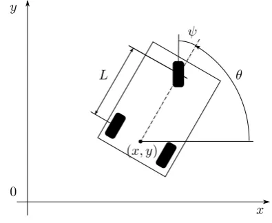
We consider a tricycle robot model.



  

˙ x ˙ y ˙ θ ˙ ψ



  

=



  

cosθ sinθ

1 Ltanψ

0



  

u1+



  

0 0 0 1



  

u2, (7)

wherexandy are the position coordinates of the center of the rear wheel axis,θis the angle between the center line of the car and the xaxis,ψ is the steering angle with respect to the car. The control inputs are represented as

u1=vscosψ

u2= ˙ψ,

where vs is the driving speed. Fig 2 shows the kinematic

model of tricycle robot. The steering angleψis constrained by

kψk ≤M, 0< M < π/2.

The constraint [8] is represented as

ψ=Mtanhw,

wherew is an auxiliary variable. Thus we get

˙

ψ=Msech2wµ2=u2,

˙ w=µ2

We substitute the equations ofψandwinto the tricycle robot model. The model is obtained as



  

˙ x ˙ y ˙ θ ˙ w



  

=



  

cosθ sinθ

1

Ltan(Mtanhw)

0



  

u1+



  

0 0 0 1



  

(3)

x y

(x, y)

θ ψ

L

[image:3.595.65.263.53.215.2]

0

Fig. 2. Kinematic model of tricycle robot

In this case, we considerη= (x, y)T _{as the output, the time}

derivative of η is calculated as

˙ η= ˙ x ˙ y =

cosθ 0 sinθ 0

u1

µ2

.

The linearized system of (8) at any points (x, y, θ, w) is clearly not controllable and the onlyu1affectsη˙. To proceed,

we need to add some integrators of the input u1. Using

dynamic compensators as

˙

u1=ν1, ν˙1=µ1,

the tricycle robot model (8) can be dynamic feedback lin-earizable. The extended model is obtained as

      ˙ x ˙ y ˙ θ ˙ w ˙ u1 ˙ ν1       =      

u1cosθ u1sinθ u1_L1 tan(Mtanhw)

0 ν1 0       +       0 0 0 0 0 1      

µ1+       0 0 0 1 0 0      

µ2 (9)

The time derivative of η˙ is calculated as

¨ η=

_L2 fh1

L2 fh2

=

ν1cosθ−u21 1

Ltan(Mtanhw) sinθ

ν1sinθ+u21 1

Ltan(Mtanhw) cosθ

,

where(h1, h2) = (x, y). Since the controller(µ1, µ2)doesn’t

appear in the equation η˙, we continue to calculate the time derivative of η¨. Then we get

η(3)=L3_fh+LgL2fhµ

=

_L3 fh1

L3_fh2

+

_L

g1L

2

fh1 Lg2L

2 fh1

Lg1L

2

fh2 Lg2L

2 fh2

µ1

µ2

. (10)

Equation (10) shows clearly that the system is input-output linearizable because state feedback control

µ=−(LgL2fh)

−1_L3

fh+ (LgL2fh)

−1_v

reduces the input-output map to y(3) ₌_v_.

The matrixLgL2fhmultiplying the modified input(µ1, µ2)

is non-singular if u1 6= 0. Since the modified input is

obtained as(µ1, µ2), the integrator with respect to the inputv

is added to the original input(u1, u2). Finally, the stabilizing

controller of the tricycle robot system (7) is presented as a dynamic feedback controller:

(

˙

u1=ν1, ν˙1=µ1,

u2=Msech2wµ2

(11)

IV. PML MODELING ANDTRACKINGCONTROLLER DESIGN OF THETRICYCLEROBOTMODEL

A. PML Model of the Tricycle Robot Model

We construct PML model of the tricycle robot system (9). The state spaces ofθandwin the tricycle robot model (9) are divided by the 13 verticesx3∈ {−π,−5π/6, . . . , π}and the

13 vertices x4 ∈ {−3.0,−2.5, . . . ,3.0}. The state variable

isx= (x1, x2, x3, x4, x5, x6)T = (x, y, θ, w, u1, v1)T.

˙ x=                

σ3+1 X

i3=σ3 wi3

3 (x3)f1(d3(i3))x5

σ3+1 X

i3=σ3 wi3

3 (x3)f2(d3(i3))x5

σ4+1 X

i4=σ4 wi4

4 (x4)f3(d4(i4))x5

0 x6 0                 +       0 0 0 0 0 1      

µ1+       0 0 0 1 0 0      

µ2.

(12)

We can construct PML models with respect tof1(x),f2(x)

and f3(x). The PML model structures are independent of

the vertex positionsx5andx6 sincex5andx6are the linear

terms. This paper constructs the PML models with respect to the nonlinear terms ofx3 andx4.

Note that trigonometric functions of the tricycle robot (9) are smooth functions and are of classC∞. The PML models are not of classC∞. In the tricycle robot control, we have to calculate the third derivatives of the outputy. Therefore the derivative PML models lose some dynamics. In this paper we propose the derivative PML models of the trigonometric functions.

B. Tracking Controller Design Using Dynamic Feedback Linearization Based on PML Model

We define the output asη= (x1, x2)T in the same manner

as the previous section, the time derivative ofηis calculated as

˙ η =

Lfph1

Lfph2 = ˙ x1 ˙ x2 =

σ3+1 X

i3=σ3 wi3

3(x3)

f1(d3(i3))x5

f2(d3(i3))x5

where the vertices are f1(d3(i3)) = cosd3(i3) and

f2(d3(i3)) = sind3(i3). The time derivative of η doesn’t

contain the control inputs (µ1, µ2). We calculate the time

derivative ofη˙. We get

¨

η1=L2fph1=

σ3+1 X

i3=σ3 wi3

3(x3)f1(d3(i3))x6

+

σ3+1 X

i3=σ3 wi3

3(x3)f10(d3(i3)) σ4+1

X

i4=σ4 wi4

4 (x4)f3(d4(i4))x25,

¨

η2=L2fph2=

σ3+1 X

i3=σ3 wi3

3(x3)f2(d3(i3))x6

+

σ3+1 X

i3=σ3 wi3

3(x3)f20(d3(i3)) σ4+1

X

i4=σ4 wi4

(4)

wheref3(d4(i4)) = tan(Mtanhd4(i4))/L. We continue to

calculate the time derivative ofη¨. We get

η(3)₁ =L3fph1+Lg1L

2

fph1µ1+Lg2L

2 fph1µ2

=x3₅

σ3+1 X

i3=σ3 wi3

3(x3)f 00

1(d3(i3)) σ4+1

X

i4=σ4 wi4

4(x4)f3(d4(i4))

!2

+3x5x6 σ3+1

X

i3=σ3 wi3

3(x3)f 0

1(d3(i3)) σ4+1

X

i4=σ4 wi4

4(x4)f3(d4(i4))

+

σ3+1 X

i3=σ3 wi3

3(x3)f1(d3(i3))µ1

+x2₅

σ3+1 X

i3=σ3 wi3

3(x3)f10(d3(i3)) σ4+1

X

i4=σ4 wi4

4(x4)f30(d4(i4))µ2,

η(3)₂ =L3_f_ph2+Lg1L

2

fph2µ1+Lg2L

2 fph2µ2

=x3₅

σ3+1 X

i3=σ3 wi3

3(x3)f 00

2(d3(i3)) σ4+1

X

i4=σ4 wi4

4(x4)f3(d4(i4))

!2

+3x5x6 σ3+1

X

i3=σ3 wi3

3(x3)f 0

2(d3(i3)) σ4+1

X

i4=σ4 wi4

4(x4)f3(d4(i4))

+

σ3+1 X

i3=σ3 wi3

3(x3)f2(d3(i3))µ1

+x2₅

σ3+1 X

i3=σ3 wi3

3(x3)f20(d3(i3)) σ4+1

X

i4=σ4 wi4

4(x4)f30(d4(i4))µ2.

The vertices f₁00(d3(i3)), f 00

2(d3(i3)) and The controller of

(12) is designed as

(µ1, µ2)T =−(LgL2fph) −1

L3fph+ (LgL

2 fph)

−1

v

=−

_L

g1L

2

fph1 Lg2L

2 fph1

Lg1L

2

fph2 Lg2L

2 fph2

−1_L3 fph1

L3 fph2

+

_L

g1L

2

fph1 Lg2L

2 fph1

Lg1L

2

fph2 Lg2L

2 fph2

−1

v

wherev is the linear controller of the linear system (13).

(

˙

z=Az+Bu,

y=Cz, (13)

wherez= (h1, Lfph1, L

2

fph1, h2, Lfph2, L

2 fph2)

T _{∈ <}6_,

A=        

0 1 0 0 0 0

0 0 1 0 0 0

0 0 0 0 0 0

0 0 0 0 1 0

0 0 0 0 0 1

0 0 0 0 0 0

       

, B=

        0 0 0 0 1 0 0 0 0 0 0 1        

, C=

        1 0 0 0 0 0 0 1 0 0 0 0         T .

Ifx56= 0, there exists a controller(µ1, µ2)T of the tricycle

robot model (12) since det(LgL2fph)6= 0.

In this case, the state space of the tricycle robot model is divided into13×13vertices. Therefore the system has12×12

local PML models. Note that all the linearized systems of these PML models are the same as the linear system (13).

In the same manner of (11), the dynamic feedback lin-earizing controller of the PML system is designed as

         ¨ u1=µ1,

u2=Msech2x4µ2,

µ1

µ2

=L3_f_ph+LgL2fhv.

(14)

The stabilizing linear controllerv =−F z of the linearized system (13) is designed so that the transfer functionC(sI− A)−1_B _{is Hurwitz.}

Note that the dynamic controller (14) based on PML model is simpler than the conventional one (11). Since the nonlinear terms of controller (14) contain not the original nonlinear terms (e.g., sinx3, cosx3, tan(Mtanhx4)) but

the piecewise approximation models.

C. Tracking Control for PML System

We apply a tracking control [15] to the tricycle robot model (7). Consider the following reference signal model

(

˙ xr=fr,

ηr=hr.

The controller is designed to make the error signal e = (e1, e2)T = η −ηr → 0 as t → ∞. The time derivative

ofe is obtained as

˙

e= ˙η−η˙r=

Lfphp1

Lfphp2

−

Lfrhr1

Lfrhr2

.

Furthermore the time derivative ofe˙is calculated as

¨

e=¨η−η¨r=

_L2 fphp1

L2 fphp2

−

L2_f

rhr1

L2 frhr2

Since the controllerµ doesn’t appear in the equation ¨e, we calculate the time derivative of¨e.

e(3)=η(3)−η(3)_r

=

_L3 fphp1

L3 fphp2

+LgL2fph µ1 µ2 −

L3_f_rhr1

L3 frhr2

The tracking controller is designed as          ¨ u1=µ1,

u2=Msech2x4µ2,

µ1

µ2

=L3fph−L

3

frhr+LgL

2 fphv.

(15)

The linearized system (13) and controller v = −F z

are obtained in the same manners as the previous sub-section. The coordinate transformation vector is z = (e1, e˙1, ¨e1, e2, e˙2, e¨2)T.

Note that the dynamic controller (15) based on PML model is simpler than the conventional one on the same reason of the previous subsection.

V. SIMULATION RESULTS

(5)

A. Ellipse-shaped reference trajectory

Consider an ellipse model as the reference trajectory.

xr1 xr2

=

R1cosθ+xr1(0) R2sinθ+xr2(0)

,

where R1 and R2 are the semiminor axes and (xr1(0), xr2(0)) is the center of the ellipse. Fig. 3 shows the simulation result. The dotted line is the reference signal and the solid line is the tricycle tracking trajectory. The semiminor parameters R1 and R2 are 10 and 25.

The initial positions are set at (x(0), y(0)) = (5,0) and

(xr(0), yr(0)) = (10,0). Fig. 4 shows the control inputsu1

andν1 of the tricycle. Fig. 5 shows the error signals of the

tricycle position(x, y).

B. Trajectory tracking control using ellipse-shaped reference models

Arbitrary tracking trajectory control can be realized using the ellipse-shaped tracking trajectory method. The controller design procedure is as follows:

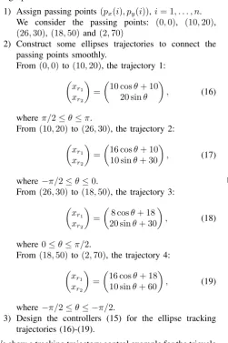
1) Assign passing points(px(i), py(i)),i= 1, . . . , n.

We consider the passing points: (0,0), (10,20),

(26,30),(18,50)and(2,70)

2) Construct some ellipses trajectories to connect the passing points smoothly.

From(0,0) to(10,20), the trajectory 1:

xr1 xr2

=

10 cosθ+ 10 20 sinθ

, (16)

whereπ/2≤θ≤π.

From(10,20)to(26,30), the trajectory 2:

xr1 xr2

=

16 cosθ+ 10 10 sinθ+ 30

, (17)

where−π/2≤θ≤0.

xr1 xr2

=

8 cosθ+ 18 20 sinθ+ 30

, (18)

where0≤θ≤π/2.

xr1 xr2

=

16 cosθ+ 18 10 sinθ+ 60

, (19)

where−π/2≤θ≤ −π/2.

3) Design the controllers (15) for the ellipse tracking trajectories (16)-(19).

We show a tracking trajectory control example for the tricycle robot system. Fig. 6 shows the reference signals (16)-(19) and the tricycle tracking trajectory. The dotted line is the reference signal and the solid line is the tricycle tracking trajectory. Fig. 7 shows the control inputs u1 andν1 of the

tricycle. Fig. 8 shows the error signals with respect to the tricycle position(x, y).

−30 −20 −10 0 10 20 30

−25 −20 −15 −10 −5

0 5 10 15 20 25

x [m]

[image:5.595.313.538.74.254.2]

y [m] (5,0) (10,0)

Fig. 3. Ellipse-shaped reference signal and the tricycle tracking trajectory

0 50 100 150 200

0.2 0.4 0.6 0.8 1

u1

0 50 100 150 200

−0.04 −0.02 0 0.02 0.04

[image:5.595.279.541.324.747.2]

ν1

Fig. 4. Control inputsu1andν1of the tricycle

0 50 100 150 200

−5 0 5

error of x

0 50 100 150 200

−5 0 5

error of y

[image:5.595.53.305.330.708.2]

t

[image:5.595.315.542.551.745.2]

(6)

−30 −20 −10 0 10 20 30 40 50 60

0 10 20 30 40 50 60 70

x [m]

y [m]

Trajectory 1 Trajectory 2

Trajectory 3 Trajectory 4

(0,0)

(10,20)

[image:6.595.60.281.73.250.2]

(26,30) (18,50) (2,70)

Fig. 6. Reference signals (16)-(19) and the tricycle tracking trajectory

0 20 40 60 80 100 120 140 160 180 200

0.2 0.3 0.4 0.5 0.6 0.7

u1

[m]

0 20 40 60 80 100 120 140 160 180 200

−0.02 −0.01 0 0.01 0.02

ν1

[m]

[image:6.595.62.561.263.765.2]

x [m]

Fig. 7. Control inputsu1 andν1 of the tricycle

0 50 100 150 200

−5 0 5

error of x [m]

0 50 100 150 200

−5 0 5

error of y [m]

time

Fig. 8. Error signals of the tricycle position(x, y)

VI. CONCLUSIONS

We have proposed a trajectory tracking controller design of a tricycle robot as a non-holonomic system with PML models. The approximated model is fully parametric. I/O dynamic feedback linearization is applied to stabilize PML control system. PML modeling with feedback linearization is a very powerful tool for analyzing and synthesizing nonlinear control systems. We also have applied a method for tracking controller to the tricycle robot. Although the controller is simpler than the conventional I/O feedback linearization controller, the tracking performance based on PML model is the same as the conventional one. Examples have been shown to confirm the feasibility of our proposals by computer simulations.

REFERENCES

[1] B. d’Andr´ea-Novel, G. Bastin, and G. Campion, “Modeling and control of non holonomic wheeled mobile robots,” inthe 1991 IEEE

International Conference on Robotics and Automation, 1991, pp.

1130–1135.

[2] R. Fierro and F. L. Lewis, “Control of a nonholonomic mobile robot: backstepping kinematics into dynamics,” inthe 34th Conference on

Decision and Control, 1995, pp. 3805–3810.

[3] T.-C. Lee, K.-T. Song, C.-H. Lee, and C.-C. Teng, “Tracking con-trol of unicycle-modeled mobile robots using a saturation feedback controller,”IEEE Transactions on Control Systems Technology, vol. 9, no. 2, pp. 305–318, 2001.

[4] J. Guldner and V. I. Utkin, “Stabilization of non-holonomic mobile robots using lyapunov functions for navigation and sliding mode control,” inthe 33rd Conference on Decision and Control, 1994, pp. 2967–2972.

[5] J. Yang and J. Kim, “Sliding mode control for trajectory tracking of nonholonomic wheeled mobile robots,”IEEE Transactions on Robotics

and Automation, pp. 578–587, 1999.

[6] B. d’Andr´ea-Novel, G. Bastin, and G. Campion, “Dynamic feedback linearization of nonholonomic wheeled mobile robot,” in the 1992

IEEE International Conference on Robotics and Automation, 1992,

pp. 2527–2531.

[7] G. Oriolo, A. D. Luca, and M. Vendittelli, “WMR control via dynamic feedback linearization: Design, implementation, and experimental val-idation,”IEEE Transaction on Control System Technology, vol. 10, no. 6, pp. 835–852, 2002.

[8] E. Yang, D. Gu, T. Mita, and H. Hu, “Nonlinear tracking control of a car-like mobile robot via dynamic feedback linearization,” in

University of Bath, UK, no. ID-218, 2004.

[9] A. D. Luca, G. Oriolo, and M. Vendittelli, “Stabilization of the unicy-cle via dynamic feedback linearization,” inthe 6th IFAC Symposium

on Robot Control, 2000.

[10] M. Sugeno, “On stability of fuzzy systems expressed by fuzzy rules with singleton consequents,”IEEE Trans. Fuzzy Syst., vol. 7, no. 2, pp. 201–224, 1999.

[11] K.-C. Goh, M. G. Safonov, and G. P. Papavassilopoulos, “A global optimization approach for the BMI problem,” inProc. the 33rd IEEE CDC, 1994, pp. 2009–2014.

[12] T. Taniguchi and M. Sugeno, “Piecewise bilinear system control based on full-state feedback linearization,” inSCIS & ISIS 2010, 2010, pp. 1591–1596.

[13] ——, “Stabilization of nonlinear systems with piecewise bilinear models derived from fuzzy if-then rules with singletons,” in

FUZZ-IEEE 2010, 2010, pp. 2926–2931.

[14] ——, “Design of LUT-controllers for nonlinear systems with PB models based on I/O linearization,” inFUZZ-IEEE 2012, 2012, pp. 997–1022.

[15] T. Taniguchi, L. Eciolaza, and M. Sugeno, “Look-Up-Table controller design for nonlinear servo systems with piecewise bilinear models,”

[image:6.595.53.284.322.499.2]