On selecting policy analysis models by forecast accuracy

Department of Economics University of Southampton Southampton SO17 1BJ UK

Discussion Papers in

Economics and Econometrics

1999

This paper is available on our website

David F. Hendry

Nuffield College,

Oxford

Grayham E. Mizon

Southampton University, UK

&

European University Institute,

Florence.

December 15, 1999

Abstract

The value of selecting the best forecasting model as the basis for empirical economic policy ana-lysis is questioned. When no model coincides with the data generation process, non-causal statist-ical devices may provide the best available forecasts: examples from recent work include intercept corrections and differenced-data VARs. However, the resulting models need have no policy implic-ations. A ‘paradox’ may result if their forecasts induce policy changes which can be used to improve the statistical forecast. This suggests correcting statistical forecasts by using the econometric model’s estimate of the ‘scenario’ change. An application to UK consumers expenditure illustrates the ana-lysis.

1 Introduction

It is a pleasure to participate in a volume celebrating the contributions to economics of Michio Mor-ishima, who was a colleague for many years. The eclectic nature of Michio’s extensive publications makes it impossible to choose any topic on which he has never written, and our chapter is related to Morishima and Saito (1964), who developed a macro-econometric model of the US economy. While Morishima and Saito (1964) focus on econometric equations with a close eye on economic-policy ana-lysis, we also consider the relationship between statistical forecasting devices and econometric models in the policy context. In particular, we investigate three aspects of this relationship. First, whether there are grounds for basing economic-policy analysis on the ‘best’ forecasting system. Secondly, whether fore-cast failure in an econometric model precludes its use for economic-policy analysis. Finally, whether in the presence of policy change, improved forecasts can be obtained by using ‘scenario’ changes, de-rived from the econometric model, to modify an initial statistical forecast. To resolve these issues, we analyze the problems arising when forecasting after a structural break (i.e., a change in the parameters of the econometric system), but before a regime shift (i.e., a change in the behaviour of non-modelled, often policy, variables), perhaps in response to the break (see Hendry and Mizon, 1998, for discussion of this distinction). These three dichotomies, between econometric and statistical models, structural breaks and regime shifts, and pre and post forecasting events, are central to our results.

We envisage a statistical forecasting system as one having no economic-theory basis (in contrast to econometric models for which this is the hallmark), so it will rarely have implications for

Financial support from the UK Economic and Social Research Council under grants R000233447 and L116251015, and the EUI Research Council, is gratefully acknowledged. We are indebted to Anindya Banerjee, Mike Clements, Jurgen Doornik, Neil Ericsson, John Muellbauer, Neil Shephard, Ian Walker and Ken Wallis, and seminar participants at Bloomington Indiana, Cambridge, IGIER, Pittsburgh, and UCL, for helpful comments.

policy analysis – and may not even entail links between target variables and policy instruments. Con-sequently, being the ‘best’ available forecasting device is insufficient to ensure any value for policy ana-lysis, and the main issue is the converse: does the existence of a dominating forecasting procedure inval-idate the use of an econometric model for policy? Our answer is almost the opposite of the Lucas (1976) critique: since forecast failure often results from factors unrelated to the policy change in question, the econometric model may continue to characterize the response of the economy to the policy, despite its forecast inaccuracy. Indeed, when policy changes are implemented, forecasts from a statistical model may be improved by combining them with the predicted policy responses from an econometric model.

The rationale for our analysis is as follows. Using the taxonomy of forecast errors in Clements and Hendry (1996a), Hendry and Doornik (1997) establish that deterministic shifts are the primary source of systematic forecast failure in econometric models. Nevertheless, there exist devices that can robus-tify forecasting models against such breaks, provided they have occurred prior to forecasting (see e.g., Clements and Hendry, 1996b, and Hendry and Clements, 1998). Such ‘tricks’ can help mitigate fore-cast failures, but the resulting models need not have useful policy implications. However, no methods are robust to unanticipated breaks that occur after forecasting, and Clements and Hendry (1998c) show that those same ‘robustifying’ devices do not offset post-forecasting breaks. Moreover, post-forecasting policy changes induce breaks in models that do not embody policy variables or links, so such models lose their robustness in that setting. Conversely, despite having experienced forecast failures from pre-forecasting breaks, econometric systems which do embody the relevant policy effects need not exper-ience a post-forecasting structural break induced by the policy-regime shift. Consequently, when both structural breaks and regime shifts occur, neither class of model alone is adequate: this suggests invest-igating whether, and if so how, they should be combined.

The structure of the analysis is as follows. In the next section, we discuss the relevant forecasting and economic-policy concepts and issues to motivate the paper. This is followed inx3 by an example

of forecasting and policy in the presence of regime shifts. We analyze the impact of structural breaks and policy changes on forecasts in an open vector equilibrium-correction mechanism inx4, and present

the case for combining the forecasts from robust statistical devices and policy-scenario changes inx5.

Section 6 then provides an extensive empirical illustration using models of UK aggregate consumption. We present conclusions inx7.

2 Background

Much previous work on economic forecasting has considered the properties of forecasts when:

1. the data generation process (DGP) is known; 2. the DGP is constant; and

3. the econometric model coincides with the DGP.

even though such mis-specified models could be beaten by other methods based on correctly-specified equations, an encompassing model – however poor – will variance-dominate in-sample, and hence also when forecasting under unchanged conditions.

Since omniscience is not characteristic of economics, a better approach assumes that none of the three conditions applies. Clements and Hendry (1994, 1998a) investigated a theory more relevant to practical economic forecasting in which:

a. the DGP is unknown;

b. the DGP is non-stationary (due to unit roots and structural breaks); and c. the econometric model is mis-specified for the DGP.

These features seem descriptive of operational economic forecasting. Moreover, they provide a rationale for ‘intercept corrections’ to model-based forecasts (see Hendry and Clements, 1994, and Clements and Hendry, 1996b), which is absent when 1.–3. hold. Further, differencing transformations, which arbit-rarily impose unit roots and thereby eliminate cointegrating relations, also change permanent structural breaks in deterministic factors into ‘blips’ (see Clements and Hendry, 1995). Thus, despite being non-optimal under 1.–3., in practice such procedures can robustify forecasts against the form of structural break that Hendry and Doornik (1997) find to be the most pernicious source of forecast failure, namely shifts in deterministic factors.

A consequence of these results is that in a class of models for processes subject to structural breaks, the best available forecasting model need not be based on the ‘causal determinants’ of the actual eco-nomic process, and as the example inx3 shows, may be based on ‘non-causal’ variables. Thus, the best

economic-policy analysis need not be based on the model that happens to forecast best, and the existence of a procedure that systematically produces better forecasts need not invalidate the policy use of another model.

The fact that a purely statistical device may provide the best available forecasts induces an appar-ent paradox. In a world characterized by a.–c. above, forecasts based on the currappar-ently-best econometric model may be beaten by statistical devices when forecasting after a structural break. Assume for the mo-ment that the statistical forecasting model does not depend on any policy variables, and hence has neither policy implications, nor produces any revisions to forecasts following policy changes. These ‘best’ fore-casts for some future period are presented to the finance minister of a given country, who thereupon de-cides that a major policy initiative is essential, and implements it. That the statistical forecasts are not then revised would justifiably be greeted with incredulity. More pertinently, providing the policy model did not fall foul of the critique in Granger and Deutsch (1992), so that changes to policy variables did indeed alter target variables, then a better forecast seems likely by adding the policy change effects pre-dicted by the econometric model to the previous forecasts. But this contradicts any claim to the effect that the statistical devices produced the best forecasts in a world of structural change.

The resolution, of course, depends on distinguishing between unknown breaks – where (e.g.) differ-encing may deliver the best achievable forecast – and known changes, the consequences of which are partly measurable. The conclusion is that a combination of robustified statistical forecasts with the scen-ario changes from econometric systems subject to policy interventions may provide improved forecasts. This is the subject ofx5.

forecasts in systems of equations. Even the (invariant) generalized forecast-error second moment cri-terion (GFESM) which they propose is not thereby unique – a monetary measure is quite conceivable (see West, 1993). Our present concern does not depend on such a difficulty, and we assume that the agent desiring the forecast has a well-specified loss measure by which to judge forecast accuracy, and there is a unique optimum for the specified criterion. However, we recognize the additional practical difficulty of determining how to evaluate the outcomes of the forecasts or the policies.

The sources of forecast errors can be categorized into six classes as discussed in Clements and Hendry (1994), for example:

(i) slope change; (ii) intercept change;

(iii) model mis-specification; (iv) parameter estimation; (v) initial forecast conditions; (vi) error accumulation.

The first two are distinguished here because their consequences seem very different in practice: zero-mean changes are not easily detected, whereas shifts in equilibrium zero-means can induce dramatic forecast failure. Such shifts need not, although they could, alter the partial derivatives of target variables with respect to instruments, in which case, the reasons for predictive failure need not impugn a policy model. Assuming they do not, e.g., because the regime shift is not due to causes that affect policy connections, then a better forecast can be derived by using the scenario change to modify the forecast obtained from a robustified method.

Alternatively, the policy model will be invalid when: a] it embodies the wrong causal attributions;

b] its target-instrument links are not autonomous;

c] its parameters are not invariant to the policy change under analysis.

These are distinct from the causes of forecast failure, though they could be a subset of the factors in any given situation. We now consider a case where poor forecasts need not invalidate policy advice.

3 Forecasting and policy analysis across regime shifts

Hendry (1997) illustrates the potential role for statistical forecasting methods when an economy is sub-ject to structural breaks, and the econometric model is mis-specified for the data generation process. He considers an economy where gross national product (GNP, denoted byy) is ‘caused’ solely by the

ex-change rate over a sample prior to forecasting, then the DGP ex-changes to one in whichyis only caused

by the interest rate, but this switch is not known by the forecaster. The DGP is non-dynamic, and in par-ticular, the lagged value ofydoes not affect its behaviour (i.e.,y

t;1is non-causal). Nevertheless, when

forecasting after the regime change, on the criterion of forecast unbiasedness, a forecasting procedure that ignores the information on both causal variables, and only usesy

t;1, namely predicting a constant

change iny byE[y t

jy t;1

] = y

t;1can outperform (in terms of bias) compared to forecasts from

mod-els which included the correct causal variable. Here, neither the statistical model, nor the econometric model based on past causal links, is useful for policy.

it would not necessarily provide good time-series forecasts in an economy subject to structural breaks that affected macroeconomic variables such as total consumers’ expenditure and inflation.

The policy implications of any given model in use may or may not change with a particular regime shift. For the setting above, if the exchange rate (e

t) did not alter when the interest rate ( r

t) was changed

in the first regime, sor

thad no direct or indirect effect on

yin that regime, then the policy implications of

the first-regime model would be useless in the second regime. That seems unlikely here, though such may well occur in practice. Ife

tis in fact altered by changes in r

t, so will y

tin both regimes. Policy analysis

involves estimation of the target-instrument responses, which in this case means@y t+h

=@r twhen

y tis

the target variable andr

tthe policy instrument. For the statistical model y

t =&

t, this response is zero

at all forecast horizons h, and so despite its robust forecasting abilities, such a model is uninformative

for policy analysis. The first-regime econometric model, on the other hand, does provide an estimate of

@y t+h

=@r

tvia (e.g.):

\ @y

t+h @r

t =

h X

i=0 @y

t+h @e

t+i @e

t+i @r

t

: (1)

In regime-2, the actual policy response is@y t+h

=@r

t, so the regime-1 econometric model policy

re-sponses in (1) will be valuable when they have the same sign, and do not over-estimate the response by more than double, whereas the statistical model is always uninformative in that it gives a zero policy response.

The next section formalizes results for forecasting in the face of both structural breaks and regime shifts, when the DGP is a cointegrated system dependent on policy-determined variables. Inx5, we

ex-plore the possibility that some combination of statistical forecasts and estimated policy responses could dominate either alone.

4 Structural breaks and regime shifts in policy models

Previous studies of the impacts on forecasting of structural breaks have looked at closed models (e.g., Clements and Hendry, 1998c, and Hendry and Clements, 1998). We now generalize these results to open models to investigate the effects of regime shifts in non-modelled variables which are often policy instru-ments. We focus on deterministic shifts following Hendry and Doornik (1997), although other paramet-ric changes could be envisaged. To establish the appropriate conditions, we first ascertain the impacts of structural breaks and regime shifts in two models. These are a second-differenced predictor (denoted DDV) and a vector equilibrium-correction mechanism (VEqCM). Clements and Hendry (1998c) show that these predictors have the same forecast biases for breaks that occur after forecasts are announced, but that the DDV is robust to deterministic breaks that have occurred before forecasting: this section draws on their approach, extending it to open models and to forecasts of growth rates (rather than levels). Thus, we consider forecasting after a structural break (due to a change in the parameters of the econometric sys-tem), but before a regime shift (here, a change in the policy rule). Since the VEqCM has some response to policy, but the DDV does not, such comparisons yield insights into the effects of using robustified forecasting methods, then exploiting policy-change information via an econometric system.

We envisage a policy rule as comprising drawings of the k policy variablesz

t from a distribution

centered on, perhaps dependent on recent past information in the economy, which we write as:

z t

=+g( I t;1

) (2)

whereE[g (I t;1

)]=0. The policy variablesz

tare under the control of a policy agency, which, within

regime, makes a drawing from (2), but when introducing a regime shift, changesto

DGP consists of the marginal process for theI(0)policy variablesz

t, and an open VEqCM, conditional

onz

t, representing the behaviour of the

nprivate-sectorI(1)variablesx t: x t = + 0 x t;1 +;z t + t where t IN n

[0;] (3)

whereandarenrof rankr. To ensure thatx tisI

(1), and notI(2), rank( 0 ?

?

)=n;r, where ?

and ?are

n (n;r)matrices such that 0 ?

=0; 0 ?

=0with(: ?

)and(: ?

)being rank-nmatrices. Also,IN

n

[0;]denotes independent drawings from ann-dimensional normal distribution

with mean zero and variance. Fort<T, theI(0)variables are stationary, so let:

E[ x t

]=; E 0 x t

=; and E[z t

]=: (4)

Taking expectations in (2) and (3):

E[x t

]== +E 0 x t

+;E[ z t

]= ++;;

using (4), so that:

=;;;; (5)

whereE[ 0

x t

]= 0

=0. From (3) and (5), therefore:

x t =+ ; 0 x t;1 ; +;z + t + t ; (6) wherez + t =z t ;.

The system in (6) can be re-written as two distinct blocks, respectively obtained on pre-multiplying by 0 and 0 ? : ; 0 x t ; = ; 0 x t;1 ; + 0 ;z + t + 0 t (7) 0 ? x t = 0 ? + 0 ? ;z + t + 0 ? t ;

where=I r

+ 0

. For explicit results under regime shifts, we assume thatz + t

does not permanently alter the growth rate of the system, so that

0 ?

;=0, or;= . We also assume that the parameters of

(2) can change freely from those of (3), although in principle, the analysis could be generalized to allow for dependencies (e.g., throughg( )depending on the disequilibria from the equilibrium corrections in

(3)), or forI(1) policy variables that entered the cointegration vectors.

The dependence assumptions made about deterministic terms are fundamental to the outcome of the following analysis. For example, if,, andwere unconnected, (6) has ‘policy ineffectiveness’, in

that only deviations ofz tfrom

have an impact, and changes inhave no effect when implemented by

keepingz + t

fixed. If so, only impulse responses would be of interest. However, we consider that shifts in

are likely to have an impact onxin practice, and hence assume,,, , andmay change freely,

withaltering in response to shifts in. Since there is no impact of changes inon,@=@ 0

= 0

entails= ; , which is an assumption of contemporaneous mean co-breaking (see Hendry, 1995b

and Hendry and Mizon, 1998), leading to = ; in (5). Thus, the final formulation in-sample

(i.e., before breaks occur) is:

x t =+ ; 0 x t;1 ; +

+ z + t

+ t

: (8)

In the face of either regime shifts or structural breaks that directly alter deterministic terms:

E[ x t ] = t (9) E 0 x t = t ; t t (10)

E[ z t

] = t

The assumption of a non-constant mean vector in (11) is essential to consider policy regime shifts, the non-constant means in (9) and (10) are required if structural breaks occur, (dependence ont), and

co-breaking in (10) is needed if mean shifts in policy are to be effective (dependence on). To the extent

that t

6= , policy will not have its anticipated consequences.

We first investigate a single structural break at timeT which shifts the DGP parameters fromto

, to

, and to

, but leavesandunchanged, such that, just prior to forecasting, the DGP

becomes: x T = + ; 0 x T;1 ; + + z + T + T (12) so: = ; ;

but the forecaster is unaware that the parameters of the DGP have changed. The changes inand

in-duce forecast failure in the VEqCM, whereas the change in reduces the predictability of policy. When thez

T+jare the realized values of the policy vectors for

j=1;2, the data outcomes are:

x T+j = + ; 0 x T+j;1 ; + + z + T+j + T+j : (13)

Ignoring estimator variances, and assuming accurate data, we consider two forecasting rules for periodT +1. One investigator uses the in-sample DGP with a provisional setting for the deviation of

the policy variablez

T+1from its mean of

to obtain the provisional 1-step forecast (called procedure

(a)): c x T+1jT =+ ; 0 x T ; +

+ z + T+1

; (14)

whereas the DDV (procedure (b)) is given by the simple rule:

g 2 x T+1jT =0;

which exploits the fact that few economic variables accelerate indefinitely, so that:

f x T+1jT =x T :

The analysis is then extended to the 2-step case, namely forecastingT+2fromT. Section 4.1 discusses

the setting of breaks where

=; policy revisions and their effects on constant parameters when

6= are discussed inx4.2, whereasx4.3 allows for both shifts. Although we focus on forecast biases, the

variances of the alternative forecasting devices are noted as these become increasingly important as the horizon increases (see e.g., Clements and Hendry, 1998c).

Since deterministic shifts induce non-stationary behaviour in all the data moments even after reduc-tion to anI(0) representation, all the moments need to be derived recursively through time, and cannot be replaced by their asymptotic equivalents. For example, whileE[

0 x T+j ] = = ; for j0, even thoughhas shifted fully to

at timeT, from (7),E[ 0 x T ]= ;(

;). These

unconditional moments are summarized in (15) when there is a structural break, but no regime shift, for

j=0;1;2.

E 0 x T;1

= ; E[ x T;1 ]=; E 0 x T+j = ; ; ;E 0 x T+j;1 = ; j+1 r ; (15) E[x T+j ] = + ; E 0 x T+j;1 ; = ; j r ; where r =

;. As = ; and

=

;

, then r

= r ;r , where r =

; andr =

; ; alsor

=

4.1 No policy revision (

=)

We first consider the forecast errors that result when the investigator is the policy maker, and setsz T+j

as a deviation from; x4.2 considers what happens whenis changed to

, where such a response could be in the light of the forecasts from either procedures (a) or (b). Sinceis unchanged, we replace

; and

;

byand

.

4.1.1 One-period ahead forecast errors

The respective forecasting errors of procedures (a) and (b), conditional on knownz

T+i, are:

b T+1jT =r ; ; r

;r z + T+1

+

T+1 (16)

whereb T+1jT

=x T+1

;bx T+1jT =x T+1 ; c x T+1jT ;and: e T+1jT =x T+1 ; f x T+1jT = 0 x T + z T+1 + T+1 : (17)

Note that although the 1-step ahead forecast errors are the same for levels and differences, this is not so for multi-step ahead forecasts. SinceE[

0 x

T;1

]=from (12), then:

E[ x T jz T+1 ;z T ]= ; ; r ; z + T ; and maintaining 0

=0(so the cointegration vectors do not trend):

0 E[x T jz T+1 ;z T ]=; 0 ; r ; z + T :

Thus, the two forecast errors have conditional means:

E b T+1jT jz T+1 ;z T =r ; ; r

;r z + T+1 ; (18) and: E e T+1jT jz T+1 ;z T =; ; 0 ; r ; z + T + z T+1 : (19) When = and

=, the DDV does worse on conditional bias ifz T+1

6=0. However, if the

VEqCM parameters change, and the policy vector does not change, soE[z T+1

] = 0, then the DDV

does better on average, noting thatE[z + T+i

]=0.

Treating thez

T+ias fixed, the respective variance matrices are:

V b T+1jT jz T+1 ;z T

=; (20)

and, for=I n ; 0 : V e T+1jT jz T+1 ;z T =+ ; 0 V 0 x T;1 ; 0 0 + 0 : (21)

Thus, the DDV always loses on variance when 6= 0. However, if is small, in the sense that the

feedbacks are slow (as is often found in practice), thenV

e

T+1jT

'2, to be compared with the bias

4.1.2 Two-periods ahead forecast errors

The last comment is not applicable to multi-step forecasts: here we focus on measuring the forecast errors in the metric of the changes, denoted byb

;T+2jT = x T+2 ; c x

T+2jT and e ;T+2jT = x T+2 ; f x

T+2jT. Setting the provisional policy vector at the value z

T+2and using (5), the 2-step ahead VEqCM

forecast is: c x T+2jT = + 0 b x T+1jT

+ z T+2 = + ; 0 x T ;

+ z + T+2 + 0 z + T+1 :

For the DDV:

f x T+2jT = f x T+1jT =x T : Since: x T+2 = + ; 0 x T+1 ; + z + T+2 + T+2 = + ; 0 x T ; + z + T+2 + 0 z + T+1 + T+2 + 0 T+1 ; as: ; 0 x T+1 ; = ; 0 x T ; + 0 z + T+1 + 0 T+1 ;

then their respective forecasting errors conditional onz T+iare:

b ;T+2jT = r ;r + ; r z + T+2 + 0 r z + T+1 + T+2 + 0

T+1 (22)

wherer

=r ;r , and:

e

;T+2jT

= ;(I r +) ; 0 r +(I r +) ; 0 ; 0 x T;1 ; + z + T+2 + 0 z + T+1 ;D z + T + T+2 + 0 T+1 ;D T ; (23)

whereD=I n ; 0 ; ; 0 2

, as2I r

+( 0

)=I r

+, and:

0 x T+1 = ; 0 ; 0 x T ; + 0 z + T+1 + 0 T+1 : Since: E 0 x T+1 ; =E 0 x T ; = 2 r ;

these have expected values:

E b ;T+2jT jz T+2 ;z T+1 =r ;r + ; r z + T+2 + 0 r z + T+1 ; and: E e ;T+2jT jz T+2 ;z T+1

=;(I r +) ; 0 r + z + T+2 + 0 z + T+1 ;D z + T :

Unconditionally, asE[z + T+i

]=0, then:

and forB=( I r +)( 0 ): E e ;T+2jT =;Br :

Conversely, if no parameters change, thenE[ b

;T+2jT

]=0= E[e

;T+2jT

]. Finally:

E b ;T+2jT ;E e ;T+2jT =r

;D(r ;r );

which could take either sign. Again treating thez

T+ias fixed, their variance matrices are:

V b ;T+2jT jz T+2 ;z T+1 =+ 0 0 (24) and: V e ;T+2jT jz T+2 ;z T+1 =BV 0 x T;1 B 0 0 ++ 0 0 +DD 0 : (25)

Thus, (25) always exceeds (24). Nevertheless, there are values for the structural breaks such that the

MSFEof (b) is less than that of (a), and we consider such cases here – otherwise, the open VEqCM is best on both bias and variance criteria, so the issue of pooling forecasts does not arise.

4.2 Policy-regime shift (

6=)

We now allow for a shift in policy regime fromto

, which only affects data from timeT+1onwards,

all other parameters remaining constant. Thus:

x T =+ ; 0 x T;1 ; +

+ z + T + T whereas x a T+j =+ ; 0 x a T+j;1 ; +

+ z T+j

+

T+j (26)

wherex a T+j

denotes the after-policy-change data. The key feature of such a policy shift is that it comes after the DDV forecasts are made, so does not alter its forecasts, whereas the VEqCM includes the policy variables, and hence produces different forecasts. We denote after-policy forecasts byc

x a T+ijT

, and let

z a T+i = +z T+i

;, so thatz T+i = z a T+i ; = z + T+i

to focus the whole change in the values of the policy variables on the regime shift for ease of comparability across cases. The unconditional moments forj=1,2are summarized in (27) when there is a regime shift, but no structural break, using

r = ;. E 0 x a T+j = ; + j r ; E x a T+j = + j;1 r : (27)

4.2.1 One-period ahead forecast errors

Now: x a T+1 =+ ; 0 x T ; +

+ z T+1

+ T+1

and as the policy maker knows the regime shift has occurred:

c x a T+1jT =+ ; 0 x T ; +

+ z T+1

so both the data and the VEqCM forecasts are shifted by the ‘policy-scenario’ difference, r . The

corresponding forecast errors, given (26), areb a T+1jT =x a T+1 ; c x a

T+1jT, so:

Equation (28) has zero conditional and unconditional expectations. The DDV remains: f x a T+1jT =x T ;

with forecast errorse a T+1jT =x a T+1 ; f x a

T+1jT, so:

e a T+1jT

= r + 0 x T + ; z T+1 ;z + T + T+1 ;

which on average equals:

E h e a T+1jT jz T+1 ;z T i

= r

+ z T+1 + 0 z + T : (29)

Compared to (19) under no structural break, the errors in (29) are increased by r

, which is also the

unconditional bias, and the additional bias relative to the VEqCM when only a regime shift occurred. The variances remain as inx4.1.1. Thus, for a pure regime shift, the VEqCM is unequivocally better.

4.2.2 Two-periods ahead forecast errors

Now: x a T+2 = + ; 0 x a T+1 ; +

+ z T+2 + T+2 = + ; 0 x T ; +

+ z T+2 + 0 z T+1 + T+2 + 0 T+1 ; as: ; 0 x a T+1 ; + = ; 0 x T ; + + 0 z T+1 + 0 T+1 :

Their 2-step ahead forecasting rules conditional onz p T+2 ,z p T+1 are respectively: c x a T+2jT = + 0 b x a T+1jT ; +

+ z T+2 = + ; 0 x T ; +

+ z T+2 + 0 z T+1 ;

whereas the DDV still uses f x

a T+2jT

=x

T. The forecast errors are denoted by b a ;T+2jT =x a T+2 ; c x a

T+2jT and e a ;T+2jT =x T+2 ; f x a

T+2jT, so that conditional on z

T+i:

b a ;T+2jT = T+2 + 0 T+1 ; and: e a ;T+2jT = ; 0 x T ; + ; ; 0 x T;1 ; + + z T+2 + 0 z T+1

; z + T + T+2 + 0 T+1 ; T :

These have expected values:

E h b a ;T+2jT jz T+2 ;z T+1 i =0; and: E h e a ;T+2jT jz T+2 ;z T+1 i

= r

+ z T+2 + 0 z T+1

;D z + T : AsE[z T+i

]=0, then:

E h e a ;T+2jT i

= r

:

4.3 Structural break and regime shift

We now allow for both the shift in policy regime fromto

, affecting data from timeT+1onwards,

and the previous deterministic shift at timeT. Now, the regime shift might be in response to the forecasts

from either the VEqCM or the DDV. Thus,x p T+j

denotes the post-break and policy-change data, for

j=1;2:

x p T+j = + 0 x p T+j;1 ; + + z T+j + T+j : (30)

We denote post-policy forecasts by c x

p

T+ijT, and let z p T+i = +z T+i

;, so thatz T+i =z + T+i as before.

4.3.1 One-period ahead

Now: x p T+1 = + ; 0 x T ; + + z T+1 + T+1 ; whereas: c x p T+1jT =+ ; 0 x T ; +

+ z T+1

: (31)

The corresponding forecast error, given (30), is (b p T+1jT =x p T+1 ; c x p T+1jT):

b p T+1jT =r

;r +r ; +z T+1 + T+1 : (32)

Equation (32) has the same conditional and unconditional expectation as (18) only when

= , since:

E h b p T+1jT jz T+1 ;z T i =r

;r +r ; +z T+1 : (33)

The DDV forecast remains:

f x p T+1jT =x T ;

with forecast errore p T+1jT =x p T+1 ; f x p T+1jT:

e p T+1jT = r + 0 x T + ; z T+1 ;z + T + T+1 ;

which on average equals:

E h e p T+1jT jz T+1 ;z T i = r ; ; 0

(r ;r )

+ z T+1 ; ; I n ; 0 z + T : (34)

Compared to (19), the errors in (34) are ‘increased’ by r

( there could be offsets between changes

in parameters). When the only structural break is a change in to

in response to the policy shift, (as in, say, the Lucas, 1976, critique), then:

E h b p T+1jT i ;E h e p T+1jT i = ; r ; r ; 0 r ;

4.3.2 Two-periods ahead Since: x p T+2 = + ; 0 x p T+1 ; + + z T+2 + T+2 = + ; 0 x T ; + + z T+2 + 0 z T+1 + T+2 + 0 T+1 ;

the respective forecasting errors conditional onz p T+2 ,z p T+1 are: c x p T+2jT = + 0 b x p T+1jT ; +

+ z T+2 = + ; 0 x T ; +

+ z T+2 + 0 z T+1 ;

for the VEqCM, as:

b x p T+1jT =x T ++ ; 0 x T ; +

+ z T+1 ; so: 0 b x p T+1jT ; + = ; 0 x T ; + + 0 z T+1 ;

and the DDV remains f x

p T+2jT

= x

T. The forecast errors are denoted by b p ;T+2jT = x p T+2 ; c x p

T+2jT and e p ;T+2jT =x T+2 ; f x p

T+2jT, so that conditional on z

T+i:

b p ;T+2jT = r

;(r ;r ) +r z T+2 + 0 r z T+1 + T+2 + 0 T+1 ; and: e p ;T+2jT = ; 0 x T ; + ; ; 0 x T;1 ; + + z T+2 + 0 z T+1 ; z + T + T+2 + 0 T+1 ; T :

These have expected values:

E h b p ;T+2jT jz T+2 ;z T+1 i =r

;( r ;r )+ ; r z T+2 + 0 r z T+1 ; and: E h e p ;T+2jT jz T+2 ;z T+1 i = ; I r ; 2

(r ;r )+ r + z T+2 + 0 z T+1 ;D z + T : AsE[z T+i

]=0, then:

E h b p ;T+2jT i =r

;( r ;r

); (35)

and: E h e p ;T+2jT i = ; I r ; 2

(r ;r )+

r

Table 1 Unconditional bias effects of structural breaks and regime shifts.

r

r r

r

r r

E h

b p T+1jT

i I

n

; 0 0

E h

e p T+1jT

i

0 ( I r

;) ;(I r

;)

;( I r

;)

E h

b p ;T+2jT

i I

n

; 0 0

E h

e p ;T+2jT

i

0 ;

I r

; 2

;

; I

r ;

2

;

; I

r ;

2

4.4 Overview

We summarize the unconditional forecast-error biases in table 1. The coefficients represent the impacts of the different breaks on the two forecasting procedures, one and two steps ahead, for growth rates. To clarify the patterns for longer horizons, the regime shift has been partitioned into the effect through any changes in the policy-reaction coefficientr , scaled by the second-regime policy mean, the policy mean

changer

, and the interaction term r r

(note that ;( I

r

;) = ;( 0

)). Since the roots of are inside the unit circle,

j

! 0asj ! 1, so in the limit, forr andr

, the DDV biases converge to the same magnitude, but the opposite sign, as the VEqCM at one-step, whereas the VEqCM biases converge to zero. Thus, only short-horizon benefits result from using the DDV as the baseline for such breaks. Conversely, the VEqCM is systematically wrong for changes in the growth rate. Finally,

the DDV biases from a regime shift converge to zero whenr =0. The table emphasises the different

susceptibilities of the two approaches to the different shifts, thereby indicating possibilities for using each to ‘correct’ the other.

5 Policy-change corrections to robust forecasts

Any need to combine two disparate models on the same information set is evidence that both are incom-plete: see Clements and Hendry (1998a). The encompassing principle argues for finding the congruent representation which can explain the failures of both models, but in the short-run that may prove infeas-ible. When the two models are differently susceptible to the causes of predictive failure, certain com-binations could be beneficial: however, the relevant combination must reflect the motivation for pooling (namely, the impacts of breaks), rather than the usual grounds as discussed in (say) Bates and Granger (1969).

5.1 Pooling policy changes and DDV forecasts

The case of interest is when the robust forecast is made from the DDV, and that prompts a policy response to change the original settingz

T+hto the actual post break and policy change outcome z

p T+h

. However, by construction, the DDV forecast is unaltered, so its forecast error changes one-for-one with the policy change. Since a deterministic shift happened one period earlier, a major change inx

T+1 would just

have occurred, inducing a correspondingly changed value forx

the VEqCM. Conversely, forecasts from the open VEqCM are revised unconditionally by the difference between (14) and (31):

E h

c x

p T+1jT

; c x

T+1jT i

= r

:

Under the assumptions used here, the change in the realization over what it would have been provision-ally, namely the difference between (13) and (30), is:

E

x p T+1

;x T+1

=

r

: (37)

If the policy-reaction matrix remained constant (

= ), the econometric model would correctly

predict the impact of the regime shift, despite the deterministic structural break. Otherwise, the policy-reaction mistake is:

r r

:

The DDV forecast error due to the policy change is equal to (37). Consequently, a combined forecast of the form:

x T+1jT

= f x

p T+1jT

+ c x

p T+1jT

; c x

T+1jT (38)

implies an unconditional forecast-error bias from (34) of ( T+1jT

=x p T+1

;x T+1jT):

E

T+1jT

=E

x

p T+1

;x T

; r

=

r r

+( I r

;)( r ;r )

;

which avoids much of the structural break, yet captures some, and possibly all, of the policy effect. This exploits the fact that the DDV is robust to the past change in the intercept, whereas the VEqCM takes account of the current change in policy. Further, as the modification from the VEqCM is deterministic, the combined procedure has the same variance as the DDV forecast would have had in the absence of policy change (

=), so after the change, for

= , (38) dominates both the DDV and the VEqCM

forecasts in mean, but loses to the latter in variance. Similarly, at two-periods ahead, let:

x T+2jT

= f x

p T+2jT

+ c x

p T+2jT

; c x

T+2jT ;

then, as:

E h

c x

p T+2jT

; c x

T+2jT i

= r

for

;T+2jT =x

p T+2

;x T+2jT:

E

;T+2jT

=

r r

+ ;

I r

; 2

( r ;r )

:

When

= , so the policy response does not change:

E

;T+2jT

= ;

I r

; 2

r =; 0

( I r

+)r ; (39)

which compares favourably with (36), and will be smaller than (35) when the roots 0

are small. As

6 Empirical illustration: DHSY revisited

Davidson, Hendry, Srba and Yeo (1978) developed an equilibrium-correction model of constant-price UK consumers’ expenditure on non-durables and services (c) as a function of real personal disposable

income (i) and annual inflation ( 4

p

t), where lower case letters denote logs and

4 =

; 1;L

4

whenL

is the lag operator. The sample period was 1959(2)–1976(2) after initial values for lags, less 8 observa-tions for forecasts. On estimating a variant of their model, our results are (all computaobserva-tions and graphics were produced by GiveWin and PcFiml: see Doornik and Hendry, 1996, 1997):

4

c t

= 0:25 (0:04)

4

i t

+ 0:24 ( 0:04)

4

i t;1

; 0:42 ( 0:11)

4

p t

+ 0:35 ( 0:11)

4

p

t;1 (40)

; 0:086 ( 0:015)

(c;i) t;4

+ 0:66 (0:22)

4

d t

;

R 2

= 0:958 b=0:0061 SC =;9:92 F

ar

(5;54) = 0:25 F arch

(4;51)=1:62 F het

(12;46)=0:81 F res

(1;58)=0:10

2 nd

(2) = 0:39 F Ch

(8;59)=0:79 V =0:092 Jt=1:31

In (40),d

tis a dummy variable associated with a pre-announced threat to change Purchase Tax, equal to

zero except in 1968(1)–(2) when it takes the values+0:01,;0:01, so its coefficient is interpretable as a

percentage change in expenditure: bdenotes the residual standard deviation, expressed as a percentage of

the level of the associated variable, and SC is the Schwarz criterion (see e.g., Hendry, 1995a). The resid-ual diagnostic tests are of the formF

j

(k;T;l), which denotes anF-test against the alternative hypothesis jfor:5

th

-order serial correlation (F

ar; see Godfrey, 1978), 4

th

-order autoregressive conditional heteros-cedasticity (F

arch; see Engle, 1982), heteroscedasticity ( F

het; see White, 1980), the RESET test ( F

res; see

Ramsey, 1969), a parameter constancy test over 1974(3)–1976(2) (FCh; see Chow, 1960), a chi-square

test for normality ( 2 nd

(2); see Doornik and Hansen, 1994), and the variance-change and joint-parameter

constancy tests from Hansen (1992) (denoted Jt and V):

and

denote significance at the 5% and 1% levels respectively. In (40), we have left

4 p

tto enter freely, rather than as part of a cointegrating relation

– which the results in Davidson et al. (1978) could be interpreted as supporting, as we wish to consider models that exclude inflation. The cointegration relationc

t ;i

tis the log of the average propensity to

consume, and so is denoted apctin the sequel. For later analyses of the performance of (40), see inter

alia Hendry and von Ungern-Sternberg (1981), Davis (1982), Birchenhall, Bladen-Hovell, Chui, Osborn and Smith (1989), Carruth and Henley (1990), Hendry, Muellbauer and Murphy (1990), Muellbauer and Murphy (1989), Harvey and Scott (1994), Hendry (1994) and Muellbauer (1994).

Here, we embed their model, denoted by the acronym DHSY, in a 3-equation VAR forc t,

i tand

4

p t

and replicate the main features of their results. Next, we drop the inflation variable from the system, and develop a model for (c

t, i

t) which reproduces the consumption-income relation, but fails on forecast tests

(and did so at the time). Thus, inflation, responding to the impact of the first ‘Oil crisis’, induced a shift in the equilibrium mean of apct, and our test period – commencing in 1974(3) – is after that shift. We also

develop a ‘time-series’ model forc

twhich does not fail on forecasting, but which would not respond to

Table 2 System goodness of fit and evaluation.

2 6 6 6 6 6 6 6 6 6 6 6 6 6 6 4

statistic c i

4

p VAR b

0:88% 2:06% 0:82% F

ar

(5;46) 0:88 2:06 0:19 F

arch

(4;43) 0:81 0:25 3:55 F

het

(32;18) 0:36 0:44 1:63

2 nd

( 2) 2:65 3:02 2:90 F

v ar

(45;101) 1:08

F v het

(192;85) 0:54

2v nd

(6) 10:6

3 7 7 7 7 7 7 7 7 7 7 7 7 7 7 5

Table 3 System residual cross correlations.

2 6 4

c i

i 0:71 ;

4

p ;0:47 ;0:31 3 7 5

the omitted variable which induced the structural break.

6.1 A three-equation VAR

The variables (c t,

i t,

4

p

t) were treated asI(1) and analyzed over the whole sample using a VAR with

5 lags, including a constant, linear deterministic trend, and 4 d

t. Table 2 shows the individual equation

and system goodness-of-fit and evaluation statistics. Vector tests are shown asF v j

(k;T ;l), and their

outcomes are consistent with a congruent system.

Table 3 records the inter-correlation structure of the residuals, which reveals important features to model in all the equations, but we will focus on those betweencand (i,

4

p). The eigenvalues of the

long-run matrix are;0:71, and;0:230:08, usingto denote p

;1to avoid confusion with income,i,

so the rank is non-zero, and is unlikely to be three given the data. The system dynamics are represented in table 4 by the eigenvalues of the companion matrix (denoted), where we also record the modulus

(jj). These eigenvalues are difficult to interpret, comprising the four roots of unity, a further unit root,

and four large complex roots, with the remainder neither zero nor unity. To understand their composition,

Table 4 System dynamics.

2 6 6 6 4

;1 ; 0:950:32 0:890:15 0:130:84 jj 1 1 1 1:00; 1:00 0:90; 0:90 0:84; 0:84

;0:510:55 ;0:48 ;0:68 0:510:26 jj 0:75; 0:75 0:48 0:68 0:57; 0:57

consider the simplest version of the VAR written as:

4

c t

= ;0:1( c;i) t;4

+v 1;t

4 i

t

= v 2;t

4 p

t

= 4

p t;1

+v 3;t

:

This system has 15 eigenvalues: six are zero, with1:0,1:0,0:974,0:974, and1, thereby

in-ducing the four roots of unity, the extra unit root, and the four large roots, with the zeroes replaced by non-zero values in table 4, corresponding to the additional short-run dynamics. Thus, despite the five unit roots, the data areI(1).

Forc

t, lags 3–5 were significant (onF(

3;49), at 5% or less), fori

t, lags 1 and 5, and for

4 p

t, only

lag 1: the trend was insignificant. As fig. 1 shows, the first two equations are constant, with their 1-step residuals having constant 95% confidence bands, but the equation for inflation is not constant: as a consequence, the system break-point Chow (1960) tests lie above the 1% critical values for a short period.

1970 1975

-.01 0 .01

Consumption

1970 1975

-.025 0 .025

Income

1970 1975

-.01 0 .01 .02

Inflation

1970 1975

.6 .8 1

Break-point Chow tests 1% line

Figure 1 System recursive graphical statistics.

6.2 Cointegration

The fitted and actual values of this system in levels have correlations of0:998,0:992and0:991, so we

turn to reductions toI(0). The cointegration analysis restricted the trend to the cointegration space, and yielded table 5 (see Doornik and Hendry, 1997, Banerjee, Dolado, Galbraith and Hendry, 1993, Jo-hansen, 1995, and Doornik, Hendry and Nielsen, 1999). For each value of the rank r of the long-run

matrix in the Johansen (1988) procedure, table 5 reports the log-likelihood values (`), eigenvalues ()

and associated maximum eigenvalue (Max) and trace (Tr) statistics together with the estimated cointeg-rating vectors (b

Table 5 Cointegration analysis.

2 6 6 6 6 6 4

r 1 2 3

` 980 986 990 0:21 0:17 0:11 Max 15:9 12:7 7:8 Tr 36:4 20:4 7:8

3 7 7 7 7 7 5 ;

2 6 6 6 6 6 4

b

1 2 3

c ;0:18 0:31 ;0:04 i 0:63 0:32 ;0:12

4

p ;0:26 ;0:38 ;0:01 3 7 7 7 7 7 5

2 6 6 6 4

b 0

c i

4

p t

1 1 ;0:68 0:45 ;0:0014 2 ;2:28 1 ;0:44 0:0063 3 ;1:93 2:40 1 ;0:0075

3 7 7 7 5

Table 6 Restricted cointegration analysis.

2 6 6 6 4

b

SE

c ;0:10 (0:036)

i 0 (;)

4

p 0 (;) 3 7 7 7 5 ;

2 6 4

c i

4 p t b

0

1 ;1 1:18 0 SE ; ; (0:21) ( ;)

3 7 5

at conventionalI(1) critical values (even ignoring the degrees-of-freedom corrections to the Tr statistic suggested by Reimers, 1992), given that (40) has a feedback coefficient with at-value of 7when the

constant is excluded, the first cointegrating vector may be a consumers’ expenditure relation. Consist-ent with this, when the trend is excluded from the cointegration relation, the coefficiConsist-ents for the income and inflation ‘elasticities’ become0:93and;0:69respectively (

2

(1)= 0:30). The sizes of the other

feedback coefficients might suggest a violation of long-run weak exogeneity, but enforcing that together with a unit income elasticity yielded

2

(4) = 6:7. The results are shown in table 6. These results are

Table 7 DHSY vector model goodness of fit and diagnostics.

2 6 6 6 6 6 4

statistic value

F v ar

(36;124) 0:79 F

v het

( 204;103) 0:93

2v nd

( 6) 11:2 F

v Ch

(24;56) 1:20 3 7 7 7 7 7 5

Table 8 DHSY vector model residual correlations.

2 6 4

c i

i 0:01 ;

4

p ;0:27 ;0:50 3 7 5

6.3 A simultaneous-equations model

A model of the system was developed by sequential simplification in fourth differences forcandi, and

first differences for 4

p, incorporating the DHSY feedback term. This yielded (41).

DHSY vector-model FIML estimates

4

c t

= 0:27 (0:08)

4

i t

+ 0:21 (0:07)

4

i t;1

; 0:22 ( 0:19)

4

p t

+ 0:14 ( 0:19)

4

p t;1

; 0:081 (0:017)

apc t;4

+ 0:67 ( 0:24)

4

d t

4

i t

= 0:69 (0:29)

4

c t;1

+ 0:53 (0:14)

4

i t;1

; 0:55 (0:12)

4

i t;4

+ 0:35 ( 0:12)

4

i t;5

+ 0:004 ( 0:006)

1

4 p

t

= 0:14 (0:08)

1

3

p t;1

+ 0:28 ( 0:07)

4

c t;2

+ 0:28 ( 0:10)

4

c t;4

; 0:17 (0:05)

4

i t;5

; 0:007 (0:002) apc

t

apc t;4

+ 4

c t

; 4

i t

(41) The likelihood-ratio test of the over-identifying restrictions on theI(0) VAR yielded

2

(38) = 44:7,

and table 7 reports the model goodness-of-fit and diagnostic statistics. On the vector diagnostic tests, the model is congruent with the sample evidence, and remains constant over the forecast period. The residual bs are0:64%, 2:00%, and0:74%: and their cross correlations for the consumption equation

are dramatically smaller than those in the VAR, consistent with finding closely similar estimates in OLS and FIML. For the rest of the paper, we treat (41) as the DGP against which to compare the remaining findings. Figure 2 reports the comparative forecast accuracy of (41), a mis-specified version which omits inflation, and a ‘time-series’ model, described in the next two sections.

6.4 A mis-specified econometric model

The natural mis-specification to consider is one where the econometrician omits inflation from the ana-lysis ofcandi, as DHSY did initially, since this induces a shift in the equilibrium mean of apc

t, causing

1960 1965 1970 1975 0

.05

Fitted and actual

1973 1974 1975 1976 0

.05

Forecasts

1960 1965 1970 1975 0

.05

1973 1974 1975 1976 0

.05 1960 1965 1970 1975 0

.05

1973 1974 1975 1976 0

.05

1974 1975 1976 -.02

0

.02 Time-series model 1974 1975 1976 -.02

0 .02

Forecast errors

Econometric model

1974 1975 1976 -.02

0

.02 DHSY

Figure 2 Fitted and actual values, 1-step forecasts, and forecast errors from all models.

Table 9 Mis-specified model statistics.

2 6 6 6 6 6 4

statistic value

F v ar

(16;94) 0:89 F

v het

(72;87) 1:03

2v nd

(4) 3:57 F

v Ch

( 16;56) 2:95

3 7 7 7 7 7 5

of analysis is close to that of the previous model, we only record the final model in (42) and its statistics.

Mis-specified model FIML estimates

4

c t

= 0:35 (0:07)

4

i t

+ 0:15 ( 0:06)

4

i t;1

; 0:049 ( 0:010)

apc t;4

+ 0:60 (0:27)

4

d t

4

i t

= 0:93 (0:33)

4

c t;1

; 0:35 ( 0:30)

4

c t;3

+ 0:45 ( 0:16)

4

i t;1

; 0:47 ( 0:14)

4

i t;4

+ 0:37 ( 0:13)

4

i t;5

+ 0:007 (0:007) apc

t

apc t;4

+ 4

c t

; 4

i t

(42)

The residual bs are0:73% and1:94%, the residual cross-correlation is;0:11and the likelihood-ratio

test of the over-identifying restrictions is 2

(16)=24:6. Table 9 reports the model goodness-of-fit and

1974 1975 1976 -.05

-.025 0 .025 .05

.075 Time-series model

1974 1975 1976

-.05 -.025 0 .025 .05

.075 Econometric model

1974 1975 1976

-.05 -.025 0 .025 .05

.075 DHSY

1974 1975 1976

-.05 -.025 0 .025 .05

.075 Econometric model with IC

Figure 3 8-step ahead forecasts of 4

c

tfrom all models.

6.5 A ‘time-series’ model

The time-series analyst is assumed to have differenced the data twice, to remove both seasonal andI(1) unit roots, and so investigates

1

4 c

t and

1

4 i

t: see Prothero and Wallis (1976). However, (43)

treats these variables as unrelated, mimicking a univariate analysis of the former to illustrate the policy analysis aspects.

‘Time-series’ model FIML estimates

1

4

c t

= 1:30 (0:32)

4

d t

b

=1:01%

1

4

i t

= 0:00 (;)

b

=2:48%

(43)

In sample, the residual standard deviations greatly exceed those of the mis-specified econometric model, and many of the diagnostic statistics reject the adequacy of this model, with some of the mis-specifications due to the moving-average error induced by over-differencing, and others perhaps to the resulting incorrectly-estimated standard errors: see table 10. However, modelling the moving-average error would lose some of the robustness to deterministic shifts (see Clements and Hendry, 1998b: also, Clements and Hendry, 1997, investigate the impact of seasonal shifts on forecasts). Despite the considerable non-congruency on these in-sample tests, the forecast test does not reject over the same period that the ‘econometric model’ failed. This reflects better forecasting and not just incorrectly-wider confidence bands, as fig. 2 shows, where the first row records the outcomes in the space of

4 c

tfor the

‘econometric model’, with the ‘time-series model’ in the second row, and the DHSY model in the third row.

Table 10 ‘Time-series’ model statistics.

2 6 6 6 6 6 4

statistic value

F v ar

( 16;104) 4:97 F

v het

( 18;147) 2:03

2v nd

(4) 6:78 F

v Ch

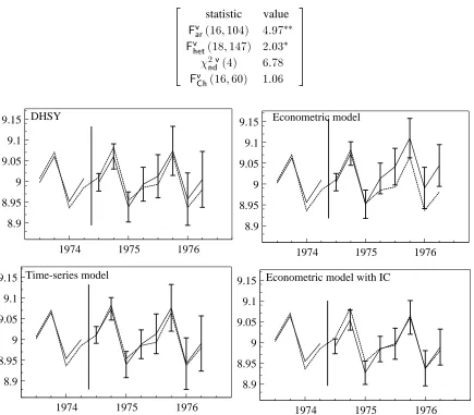
( 16;60) 1:06 3 7 7 7 7 7 5

1974 1975 1976

8.9 8.95 9 9.05 9.1

9.15 DHSY

1974 1975 1976

8.9 8.95 9 9.05 9.1

9.15 Time-series model

1974 1975 1976

8.9 8.95 9 9.05 9.1

9.15 Econometric model

1974 1975 1976

8.9 8.95 9 9.05 9.1

9.15 Econometric model with IC

Figure 4 8-step ahead forecasts forc

tfrom all models.

to mimic the role of an ‘exogenous’ policy variable). Thus, it may be possible to beat the ‘time-series’ forecasts in such a setting, asx6.7 considers.

6.6 Dynamic forecasts

The above analysis recorded the sequence of1-step forecasts, so we now evaluate the forecast

perform-ances on8-step forecasts, including an attempt to intercept correct (IC) the ‘econometric’ model using the

residual at the forecast origin to set it back on track (see Clements and Hendry, 1996b). The outcomes for

4

c

tare shown in fig. 3, and for levels in fig. 4. The IC improves the mis-specified econometric model,

but would have worsened DHSY if also used there.

These8-step results are after the break induced by the oil crisis, so we also record12-step forecasts

1973 1974 1975 1976 8.9

9 9.1

9.2 Time-series model

1973 1974 1975 1976 8.9

9 9.1

9.2 Econometric model

1973 1974 1975 1976 8.9

9 9.1

9.2 DHSY

1973 1974 1975 1976 8.9

9 9.1 9.2

Econometric model with IC

Figure 5 12-step ahead forecasts forc

tfrom all models.

1972 1973 1974 1975 1976 1977 8.9

9 9.1

c

1972 1973 1974 1975 1976 1977 9.2

9.3 9.4

i

1972 1973 1974 1975 1976 1977 .1

.2 ∆4p

1972 1973 1974 1975 1976 1977 0

.025 .05

∆4c

1972 1973 1974 1975 1976 1977 -.05

0 .05 .1

∆4i

1972 1973 1974 1975 1976 1977 -.35

-.3 -.25 -.2

c-i

New data Original data

Figure 6 Original and post-policy data forc,y, 4

p,c;y, 4

cand 4

6.7 Post-policy forecasts

The final stage was to construct the data that would have resulted after a substantial policy change aimed at preventing the large fall in income and expenditure that actually occurred. To simulate a large income-tax reduction, income was increased by 2.5%, over what it would otherwise have been, by adding 0.025 toiusing an indicator variable for the remainder of the forecast period. The data on

4

p,iandcwere

sequentially generated, observation by observation, using the coefficients in (41) and adding on its resid-uals. Thus, had the policy indicator been zero, the original data would have been reproduced precisely by this process. Figure 6 compares the original and post-policy data, showing that the policy successfully raised expenditure, but also induced some additional inflation from the cross-equation feedbacks.

Next, each of the four models was used to forecast this altered future data. We already know that the time-series forecasts are unaltered, so those errors change to the extent the data are shifted. The DHSY and mis-specified econometric models include the policy dummy with an imposed coefficient of unity. The IC model needed two non-zero periods before the forecast to avoid perfect collinearity with the policy indicator, but otherwise was unaltered. Figure 7 records the four sets of8-step forecasts. The

time-series forecasts remain useful, especially compared to those from the econometric model, and the great improvement from intercept-correcting the latter is obvious.

1974 1975 1976

-.05 0 .05 .1

DHSY

1974 1975 1976

-.05 0 .05

.1 Time series

1974 1975 1976

-.05 0 .05

.1 Econometric model

1974 1975 1976

-.05 0 .05

.1 Econometric model with IC

Figure 7 8-step ahead forecasts of 4

c

tfrom all models on the post-policy data.

the DHSY DGP.

1974 1975 1976 1977

.01 .02 .03 .04

∆4c

1974 1975 1976 1977

.02 .04 .06

Econometric model

c

1974 1975 1976 1977

-.06 -.04

-.02 c-i

DHSY

∆4c

Figure 8 Comparative policy responses of DHSY and econometric model.

Figure 9 reports the forecast errors from all the methods for comparison.

1974 1975 1976

-.075 -.05 -.025 0

.025 DHSY

Original data

Policy-modified data

1974 1975 1976

-.075 -.05 -.025 0 .025

Time-series model

1974 1975 1976

-.075 -.05 -.025 0 .025

Econometric model

IC

no IC

1974 1975 1976

-.075 -.05 -.025 0

.025 Time series model with scenario effects

without IC

with IC

Figure 9 8-step ahead forecast errors from all models on the post-policy data for 4 c

Original Data

Model DHSY Ect TS IC

Mean ;1:54 ;2:64 ;0:75 ;0:10

SD 2:58 2:84 1:36 2:35

New Data

Model DHSY Ect TS IC TS(+Ect) TS(+IC) Mean ;1:92 ;3:53 1:48 ;0:68 ;1:61 ;1:31

SD 2:85 3:20 1:21 2:46 1:45 1:73

Table 11 8-period ahead forecast-error means and standard deviations.

There is a clear benefit from the new form of intercept correction relative to the econometric models’ forecasts, and the accuracy is close to that achieved by the extended DHSY system. However, the time-series forecasts remain accurate even if not corrected. Table 11 records the percentage forecast errors and their standard deviations (TS, Ect, and DHSY, respectively denote (43), (42) and (41); IC is the intercept-corrected econometric model; TS(+Ect) is the scenario-intercept-corrected TS forecast based on adding the dif-ference between the Ect based on the new and the original data, and TS(+IC) is the scenario-corrected TS using the difference between the IC based on the new and original data.1

Thus, for the new data TS is the most accurate, with IC close, and on mean forecast error, the latter does best. Both TS(+Ect) and TS(+IC) perform reasonably, but do not dominate because the policy shift happens to induce an insigni-ficant positive bias in TS (see fig. 9c). It is interesting how poorly the DHSY forecasting model performs, given it is the DGP.

Original Data

Model DHSY Ect TS IC Mean 0:67 ;0:28 0:36 1:91

SD 1:40 1:71 0:80 1:24

New Data

Model DHSY Ect TS IC TS(+Ect) TS(+IC) Mean 0:55 ;0:77 2:27 1:45 ;0:10 ;0:07

SD 1:49 1:80 1:27 1:28 0:87 0:84

Table 12 4-period ahead forecast-error means and standard deviations.

Differences are more dramatic when the first four-period ahead forecasts are considered as in table 12. Now, for the new data TS(+IC) is a clear winner, closely followed by TS(+Ect), with TS on the original data next best. Thus, the scenario corrections can be useful in modifying a statistical device for forecast-ing.

1

7 Conclusion

The main conclusions relate to the three issues posed in the introduction. The dominance in forecasting of an econometric policy model by a purely statistical device is not sufficient to sustain the use of the lat-ter for policy: a statistical forecasting procedure which embodies no links between target variables and policy instruments has no implications for economic policy analysis, so outperforming on forecasting is clearly insufficient to justify policy analysis. Further, since the sources of forecast failure may be unre-lated to the policy issue under analysis, forecast dominance does not by itself demonstrate the invalidity of the econometric model for the policy: the empirical example illustrated this proposition. However, combining robustified forecasts with policy-scenario changes may dominate either alone in a world sub-ject to regime shifts: forecasting procedures designed to be robust to deterministic shifts that have oc-curred prior to forecasting could be improved by ‘intercept correcting’ them using the policy-change effects entailed by the econometric model. For short-horizon forecasts, the UK consumers’ expenditure model illustrated this result. These findings exploited the different forecast biases of the various models to breaks pre and post forecasting, discussed in Hendry and Clements (1998) and Clements and Hendry (1998c), but ignored the variance consequences.

The present paper is more in the form of an existence theorem for the combination of robust fore-casts and policy-change corrections than a practical manifesto, in that we have not yet developed criteria for when the proposal will outperform. The usual ‘combination of forecasts’ approach (see e.g., Bates and Granger, 1969, Diebold, 1989, and Coulson and Robins, 1993) does not seem appropriate, since in-sample correlations between forecast errors are unlikely to be a useful guide when deterministic shifts occur. Moreover, the corrections proposed above involve the difference between two dynamic forecasts of the econometric model, and not simply its second set of forecasts. A first step would be to determ-ine when a deterministic shift occurred just before the forecast origin, and we are currently developing directed tests for such an event. That would enhance the decision to adopt a robust device. A second step would involve checking if the policy predictions from the econometric system remained reliable in the face of the shift, which is bound to involve judgement, perhaps supported by the results of tests of parameter invariance to previous shifts (see e.g., Favero and Hendry, 1992, Engle and Hendry, 1993, and Ericsson and Irons, 1995), and of the policy relevance of the model (see Granger and Deutsch, 1992). We have assumed that the in-sample econometric model coincides with the DGP, and allowing for model mis-specification and estimation must weaken the results. An alternative we are also investigating is us-ing the time-series forecasts to ‘intercept correct’ the post-policy forecasts of the econometric model: as analyzed in Clements and Hendry (1998d), this may provide a useful route to avoiding forecast failure when structural breaks and regime shifts occur.

References

Banerjee, A., Dolado, J. J., Galbraith, J. W., & Hendry, D. F. (1993). Co-integration, Error Correction and the Econometric Analysis of Non-Stationary Data. Oxford: Oxford University Press.

Bates, J. M., & Granger, C. W. J. (1969). The combination of forecasts. Operations Research Quarterly,

20, 451–468.

Birchenhall, C. R., Bladen-Hovell, R. C., Chui, A. P. L., Osborn, D. R., & Smith, J. P. (1989). A seasonal model of consumption. Economic Journal, 99, 837–843.

Chow, G. C. (1960). Tests of equality between sets of coefficients in two linear regressions. Economet-rica, 28, 591–605.

Clements, M. P., & Hendry, D. F. (1993). On the limitations of comparing mean squared forecast errors. Journal of Forecasting, 12, 617–637. With discussion.

Clements, M. P., & Hendry, D. F. (1994). Towards a theory of economic forecasting. In Hargreaves, C. (ed.), Non-stationary Time-series Analysis and Cointegration, pp. 9–52. Oxford: Oxford Uni-versity Press.

Clements, M. P., & Hendry, D. F. (1995). Macro-economic forecasting and modelling. Economic Journal, 105, 1001–1013.

Clements, M. P., & Hendry, D. F. (1996a). Forecasting in macro-economics. In Cox, D. R., Hinkley, D. V., & Barndorff-Nielsen, O. E. (eds.), Time Series Models: In econometrics, finance and other fields. London: Chapman and Hall.

Clements, M. P., & Hendry, D. F. (1996b). Intercept corrections and structural change. Journal of Applied Econometrics, 11, 475–494.

Clements, M. P., & Hendry, D. F. (1997). An empirical study of seasonal unit roots in forecasting. In-ternational Journal of Forecasting, 13, 341–355.

Clements, M. P., & Hendry, D. F. (1998a). Forecasting Economic Time Series: The Marshall Lectures on Economic Forecasting. Cambridge: Cambridge University Press.

Clements, M. P., & Hendry, D. F. (1998b). Forecasting Non-stationary Economic Time Series: The Zeuthen Lectures on Economic Forecasting. Cambridge, Mass.: MIT Press. Forthcoming.

Clements, M. P., & Hendry, D. F. (1998c). On winning forecasting competitions in economics. mimeo, Institute of Economics and Statistics, University of Oxford.

Clements, M. P., & Hendry, D. F. (1998d). Using time-series models to correct econometric model fore-casts. mimeo, Institute of Economics and Statistics, University of Oxford.

Coulson, N. F., & Robins, R. P. (1993). Forecast combination in a dynamic setting. Journal of Forecast-ing, 12, 63–68.

Davidson, J. E. H., Hendry, D. F., Srba, F., & Yeo, J. S. (1978). Econometric modelling of the aggreg-ate time-series relationship between consumers’ expenditure and income in the United Kingdom. Economic Journal, 88, 661–692. Reprinted in Hendry, D. F. (1993), Econometrics: Alchemy or Science? Oxford: Blackwell Publishers.

Davis, E. P. (1982). The consumption function in macroeconomic models: A comparative study. Dis-cussion paper 1, Bank of England. Technical Series.

Diebold, F. X. (1989). Forecast combination and encompassing: Reconciling two divergent literatures. International Journal of Forecasting, 5, 589–592.

Doornik, J. A., & Hansen, H. (1994). A practical test for univariate and multivariate normality. Discus-sion paper, Nuffield College.

Doornik, J. A., & Hendry, D. F. (1996). GiveWin: An Interactive Empirical Modelling Program. London: Timberlake Consultants Press.

Doornik, J. A., & Hendry, D. F. (1997). Modelling Dynamic Systems using PcFiml 9 for Windows. Lon-don: International Thomson Business Press.

Doornik, J. A., Hendry, D. F., & Nielsen, B. (1999). Inference in cointegrated models: UK M1 revisited. Journal of Economic Surveys, 12, 533–572.

United Kingdom inflations. Econometrica, 50, 987–1007.

Engle, R. F., & Hendry, D. F. (1993). Testing super exogeneity and invariance in regression models. Journal of Econometrics, 56, 119–139. Reprinted in Ericsson, N. R. and Irons, J. S. (eds.) Testing Exogeneity, Oxford: Oxford University Press, 1994.

Ericsson, N. R., & Irons, J. S. (1995). The Lucas critique in practice: Theory without measurement. In Hoover, K. D. (ed.), Macroeconometrics: Developments, Tensions and Prospects. Dordrecht: Kluwer Academic Press.

Favero, C., & Hendry, D. F. (1992). Testing the Lucas critique: A review. Econometric Reviews, 11, 265–306.

Godfrey, L. G. (1978). Testing for higher order serial correlation in regression equations when the re-gressors include lagged dependent variables. Econometrica, 46, 1303–1313.

Granger, C. W. J., & Deutsch, M. (1992). Comments on the evaluation of policy models. Journal of Policy Modeling, 14, 497–516.

Hansen, B. E. (1992). Testing for parameter instability in linear models. Journal of Policy Modeling,

14, 517–533.

Harvey, A. C., & Scott, A. (1994). Seasonality in dynamic regression models. Economic Journal, 104, 1324–1345.

Hendry, D. F. (1979). Predictive failure and econometric modelling in macro-economics: The transac-tions demand for money. In Ormerod, P. (ed.), Economic Modelling, pp. 217–242. London: Heine-mann. Reprinted in Hendry, D. F. (1993), Econometrics: Alchemy or Science? Oxford: Blackwell Publishers.

Hendry, D. F. (1994). HUS revisited. Oxford Review of Economic Policy, 10, 86–106.

Hendry, D. F. (1995a). Dynamic Econometrics. Oxford: Oxford University Press.

Hendry, D. F. (1995b). A theory of co-breaking. Mimeo, Nuffield College, University of Oxford.

Hendry, D. F. (1997). The econometrics of macro-economic forecasting. Economic Journal, 107, 1330– 1357.

Hendry, D. F., & Clements, M. P. (1994). Can econometrics improve economic forecasting?. Swiss Journal of Economics and Statistics, 130, 267–298.

Hendry, D. F., & Clements, M. P. (1998). Economic forecasting in the face of structural breaks. In Holly, S., & Weale, M. (eds.), Econometric Modelling: Techniques and Applications. Cambridge: Cambridge University Press. Forthcoming.

Hendry, D. F., & Doornik, J. A. (1997). The implications for econometric modelling of forecast failure. Scottish Journal of Political Economy, 44, 437–461. Special Issue.

Hendry, D. F., & Mizon, G. E. (1998). Exogeneity, causality, and co-breaking in economic policy analysis of a small econometric model of money in the UK. Empirical Economics, 23, 267–294.

Hendry, D. F., Muellbauer, J. N. J., & Murphy, T. A. (1990). The econometrics of DHSY. In Hey, J. D., & Winch, D. (eds.), A Century of Economics, pp. 298–334. Oxford: Basil Blackwell.

Hendry, D. F., & von Ungern-Sternberg, T. (1981). Liquidity and inflation effects on consumers’ ex-penditure. In Deaton, A. S. (ed.), Essays in the Theory and Measurement of Consumers’ Beha-viour, pp. 237–261. Cambridge: Cambridge University Press. Reprinted in Hendry, D. F. (1993), Econometrics: Alchemy or Science? Oxford: Blackwell Publishers.