Abstract—In this paper, a new multiclass classification method has been proposed. During the training process, the simple linear regression was used to find the linear relationship between the paired variables as well as its centroid on every class. The three points: based on linear functions, centroids, and input values, were used to find the class membership of the presented new object by using the formula in calculating the area of triangle. Four standard and public datasets taken from UCI machine learning repository were used to evaluate the performance of the proposed algorithm using 5-fold cross-validation. Empirical results show the satisfactory performance of XAC algorithm on linearly and nonlinearly separable classes with small training size and/or high dimension.
Index Terms—data mining, multiclass classification, simple linear regression, geometric properties
I. INTRODUCTION
ncovering hidden useful knowledge within large datasets is the main goal of data mining. It helps people in making proactive and knowledge driven decisions. Hence, various data mining techniques emerged in different research topics like sequential rules, pattern recognition, clustering, regression and classification.
Among these topics, data classification became one of major researches due to its wide applications [1][3], such as in biomedical modeling, biological modeling and etc. Classification is a supervised learning method that refers to the task of analyzing a set of data containing observations in order to learn a model or function that can be used in identifying the new observation into one of the predefined classes. It has been an active research topic not only in the machine learning area, but also in statistics [2]. Early work on classification focused on finding which variables discriminate between two or more classes, or also known as discriminant function analysis (DFA). The underlying idea in DFA is to use the predictor variables from the training set to construct the discriminant functions, like linear functions, that will determine the group membership of the unseen
Manuscript received May 22, 2015; revised July 20, 2015.
Jeremias T. Lalis is an Assistant Professor in the College of Computer Studies and the Director of the Institutional Research and Publication Office of La Salle University, Ozamiz City, Philippines, e-mail: [email protected]
object. Modern classification approaches focused on automatic generation of rule (e.g. decision tree), the use of conditional probabilities ( e.g. Naïve Bayes), calculating the distances in the feature space (e.g. K-nearest neighbor), and even through linear and nonlinear regression (e.g. support vector machine) in creating more flexible models.
In this paper, the researcher presents a new and simple classification method based on simple linear regression in finding the linear relationships between the object’s attributes and to use its geometrical properties, area of triangle, in calculating the distance of the new object from the predetermined classes. This study also shows the applicability of simple linear regression in linear and nonlinear separable multiclass classification problems. Four standard datasets from the UCI machine learning repository were used to measure and evaluate the performance of the proposed algorithm.
II. RELATED WORK
A. Simple Linear Regression
Linear regression is the task of finding the best-fitting straight line, or also known as regression line, through the feature space [12]. The main idea in this technique is to reveal the linear relationship or to derive a linear function that links variable x and y, denoted as
b mx
y (1)
where y is the criterion variable, m is the slope, x is the predictor variable, and b as y-intercept of the trendline.
In this case, the value of variable y is predicted based only on variable x, thus, it is called as simple linear regression. There are some other linear and binary classification methods that apply this technique to classify linearly separable classes, such as perceptron and support vector machines (SVM). However, the best-fitting line in these methods is used to separate the two classes, wherein it is called as hyperplane.
B. Linear Classification via Hyperplane
Regression and classification are both learning techniques in data mining that are used to create predictive models based on the presented data. However, these methods produce different values for output variables, and thus, used
X-Attributes Classifier (XAC): A New
Multiclass Classification Method by Using
Simple Linear Regression and Its Geometrical
Properties
Jeremias T. Lalis, Member, IAENG
differently. Since regression takes continuous values as output, then it is used to estimate or predict a response. On the other hand, classification takes class labels as output so it is used to find the class membership of the object. However, there are some classification methods, like perceptron and SVM, that adopted the concept of linear regression to classify objects but in a different and far more complex manner.
Perceptron
Perceptron is one of the earliest algorithms for linear classification invented by Frank Rosenblatt at the Cornell Aeronautical Laboratory in 1957 [4]. It is also considered as a simple model of neuron that has a set of external input x that can be of any number, an internal input b, and one Boolean output value. The main idea in this method is to find the suitable values for the weights w in the separating hyperplane, f(x), so that the training examples are correctly classified. The hyperplane is geometrically defined as
otherwise b x w if x f 0 0 1 ) ( (2)
However, the separating hyperplane is only guaranteed to be found if the learning set is linearly separable, otherwise, the training process will never stop. This major drawback makes this algorithm less applicable to many pattern recognition problems.
Support Vector Machine (SVM)
Like perceptron, support vector machine (SVM) is a hyperplane based classifier, but it is backed with solid theoretical grounding [5]. The objective in this method is to find an optimal hyperplane, w.x + b = 0, that separates the two classes with the largest margin. It means that this hyperplane has the largest minimum distance to the training set. The hyperplane can be formally defined as
) (
)
(x sign w x b
f T (3)
where w is the weight vector and b as the bias which can be computed based on the training data point by solving a constrained quadratic optimization problem. The final decision can then be derived and defined as
b x x y sign x f i N i i i ( ) )(
1
(4)
Wherein this function depends on a non-zero support vectors αi which are often a small fraction of the original
dataset.
III. XACALGORITHM
The main objective of this study is to use the linear function, f(x) = m.x + b, in classifying linear and nonlinear separable multiclass objects. In general, the proposed algorithm has two stages, the training phase and classification phase.
A. Training Phase
In order for any classifier to identify the correct class membership of the new object, it should be trained first using the training set and create a predictive model. Fig. 1 shows the block diagram of x-attributes classifier (XAC) training procedure.
1) Given the training dataset with n number of x attributes and k tuples, find the linear relationship between the pairs of attributes in each class j,
1 1 1 1 2 2 2 2 1 1 1 1 ) ( ... ) ( ) ( n n n n j j j x x f x x f x x f (5)
where fj(xi) is the linear function between attributes xi
and xi+1, αi is the slope, and βi is the offset.
The slope αi in fj (xi) can be computed as:
2 2 1 1) ( i i i i i i i x x k x x x x k (6)while the offset βi in fj(xi) is computed as:
k x
xi i i
i
1 (7)
The resulting values of α and β between the paired attributes in each class will then be used as internal inputs to calculate the output value during the classification stage. 2) Calculate the centroid C of the paired variables xi and
xi+1 for each class j, denoted as C j (
x
i ,x
i1): [image:2.595.308.557.177.419.2]n x x
n x
x i
i i
i
1
1
, (8)
Figs. 2, 3 and 4 illustrate the scatter plot of each pair of attributes as well as its corresponding regression line for each class in the Iris flower dataset.
B. Classification Phase
After the training process, the resulting model can now be used to classify the new object. Fig. 5 shows the
classification process of XAC algorithm.
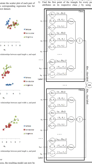
To determine the class membership of the input object: 1) Find the first point of the triangle for every paired
attributes on its respective class j by using the
Fig. 4. Scatter plot and linear relationships between petal length x3 and petal
[image:3.595.143.534.83.776.2]width x4 of the three classes.
Fig. 3. Scatter plot and linear relationships between sepal width x2 and petal
[image:3.595.62.294.145.299.2]length x3 of the three classes.
Fig. 2. Scatter plot and linear relationships between sepal length x1 and sepal
width x2 of the three classes.
[image:3.595.62.289.552.705.2]previously calculated linear functions fj(x1), fj(x2), fj(x3),
…, fj(xn-1) and its corresponding input values x1, x2, x3,
…, xn-1. The resulting xy-coordinates would be on the
form of (external input xi, internal input f(xi)).
2) The previously computed centroid C on each paired attribute in class j will serve as the second point of the corresponding triangles, in the form of (internal input
i
x
, internal inputx
i1).3) Pair the input values, e.g. (external input x1, external
input x2), to obtain the third point of the corresponding
triangles in class j.
4) Use the three points on each paired attributes in class j to calculate the area of its corresponding triangles,
( )
2) ( Area 1 1 1 1 i n i n i i i i i i x x f x x f x x x x x (9)
5) Calculate the distance of the input object from the feature vectors in every class j by summing up all the corresponding ∆Area of its paired attributes,
1 1 Area n i i j dist (10)where n is the number of attributes.
6) The class that obtained the least distance will be declared as the winner or the class membership of the new object.
IV. EXPERIMENTS
A. Dataset
To measure and validate the performance of the proposed algorithm, four public datasets from UCI Machine Learning Repository were considered: Iris Flower [6], Wheat Seed Kernel [7], Breast Tissue [8], Breast Cancer Wisconsin (Diagnostic) [9], and One Hundred Plant Species Leaves [10]. Table I shows the characteristics of each dataset used in the experiments.
B. Evaluation
To evaluate the performance of the proposed method, 5-fold cross-validation was used in each experiment. The training and testing steps were performed five times by
partitioning the dataset into five mutually exclusive subsets or folds. Accuracy, precision, recall and F score were also used to measure the correctness, exactness, completeness, and retrieval performance, respectively, of the model being produced by XAC in every experiment.
V. RESULTS AND DISCUSSION
The summary of experiments results using the four datasets is reported in Table II.
As we can see, the XAC algorithm performs best with the Iris flower dataset compared with the other three datasets. The result proves the applicability of simple linear regression in classifying not only linearly separable, but
including nonlinearly separable classes. Next to it are the results of the experiments conducted with the breast cancer dataset having a mean precision of 89.92%. Note that the division of the dataset, training and testing, is slightly imbalanced, wherein 62% is coming from the benign class and the rest is from the malignant class. However, results from the experiments using the wheat seed dataset are far more better in terms of mean accuracy, mean recall, and mean F-score compared to the results with the breast cancer dataset.
It is also notable that the algorithm was able to produce an acceptable result for leaves dataset in terms of precision at 86.47% despite of the limited number of training set, three per class, and high dimensionality. Adding to the difficulty of the classification problem in this dataset is that many of the sub species resemble close appearance with the other major species, and many sub species resemble a radically different appearance with its major specie [11]. Furthermore, results also show the robustness of the approach by using only the shape-based dataset during training and testing.
However, results given by XAC using the breast tissue dataset give the lowest result, especially in terms of completeness at 67.88%. This is due to the imbalance on the number of training and testing sets in each class, wherein, 48% of the total number of it is coming from one class only. In general, the proposed algorithm performs satisfactorily even with small number of training set at 20% of the total size on each dataset.
VI. CONCLUSION
This paper has presented a new method that can be used for multiclass classification problems with linearly and nonlinearly separable classes using simple linear regression which is originally designed for binary classification
TABLEI DATASET CHARACTERISTICS
Dataset Training Size Testing Size Classes # of Dim Iris Flower 10 per class 40 per class 3 4 Wheat Seed 14 per class 56 per class 3 7 Breast Tissue 4 for class 1
10 for class 2 3 for class 3 4 for class 4
17 for class 1 39 for class 2 11 for class 3 18 for class 4
4 4
Breast Cancer 71 for class 1 42 for class 2
286 for class 1 170 for class2
2 30 Leaves-Shape 3 per class 13 per class 25 64
TABLEII
EXPERIMENTS RESULTS SUMMARY
problem with linearly separable classes only. Empirical results from the experiments conducted using the four standard and public datasets taken from UCI machine learning repository showed the satisfactory performance of the proposed algorithm.
For the future work, several avenues for improvement can still be considered like using the nonlinear regression to cater those paired attributes with nonlinear relationship.
REFERENCES
[1] V. S. M. Tseng and C. Lee, “Cbs: A new classification method by using sequential patterns,” in Proc.2005 SIAM International Data
Mining Conference, CA, 2005, pp.596-600.
[2] A. An, Classification methods. CA: Idea Group Inc, 2005, pp. 1-6. [3] A. Arakeiyan, L. Nerisyan, A. Gevorgyan, and A. Boyajyan,
“Geometric approach for Gaussian-kernel bolstered error estimation for linear classification in computational biology,” International
Journal “Information Theories and Applications”, vol. 21, no. 2, pp.
170-181-, 2014.
[4] F. Rosenblatt, “The perceptron-a perceiving and recognizing automation,” Cornell Aeronautical Laboratory, New York, Report 85-460-1, 1957.
[5] C. Cortes and V. Vapnik, “Support-vector networks,” Machine
Learning, vol. 20, no. 3, pp. 273-297, 1995.
[6] UCI Machine Learning Repository, “Iris data set,” 1988. [Online]. Available: archive.ics.uci.edu/ml/datasets/Iris
[7] UCI Machine Learning Repository, “Seeds data set,” 2012. [Online]. Available: archive.ics.uci.edu/ml/datasets/seeds
[8] UCI Machine Learning Repository, “Breast tissue data set,” 2010. [Online]. Available: archive.ics.uci.edu/ml/datasets/Breast+Tissue [9] UCI Machine Learning Repository, “Breast cancer wisconsin
(diagnostic),” 1995. [Online]. Available: archive.ics.uci.edu/ml/datasets/Breast+Cancer+Wisconsin+(Diagnosti c)
[10] UCI Machine Learning Repository, “One-hundred plant species leaves data set,” 2012. [Online]. Available:
archive.ics.uci.edu/ml/datasets/One-hundred+plant+species+leaves+data+set
[11] C. Mallah, “Probabilistic Classification from a K-Nearest-Neighbor Classifier,” Computational Research, vol. 1, no. 1, pp. 1-9, 2013. [12] Wikipedia, “Linear regression,” 2015. [Online]. Available: