Fast Learning Algorithm for Fuzzy Inference Systems using Vector Quantization

Fast Learning Algorithm for Fuzzy Inference

Systems using Vector Quantization

Hirofumi Miyajima

†1

, Noritaka Shigei

†2

, and Hiromi Miyajima

†3

Abstract—It is known that learning methods of fuzzy in-ference systems using vector quantization (VQ) and steepest descend method (SDM) are superior in terms of the number of rules. However, they need a great deal of learning time. The cause could be that both of VQ and SDM perform only local searches. On the other hand, it has been shown that a learning method of radial basis function (RBF) networks using VQ and generalized inverse method (GIM) is much fast. In this paper, we propose a new learning method using VQ, GIM and SDM. The method iterates three stages in the outer loop of the algorithm. The first stage adjust the fuzzy rule arrangement by using VQ, the second one determines the weights of fuzzy rules by using GIM, and the third one updates both of the rule arrangement and the weights. In order to demonstrate the validity of the proposed method, numerical simulations for function approximation and pattern classification problems are performed. Specifically, it is shown that the proposed method reduces the learning time to about one-tenth compared to conventional methods in function approximation problem.

Index Terms—Fuzzy Inference Systems, Vector Quantiza-tion, Neural Gas, Generalized Inverse Method, Appearance frequency.

I. INTRODUCTION

Many studies on self-tuning fuzzy systems have been made [1]–[3]. Their aim is to construct automatically fuzzy systems from learning data. Although most of the methods are based on steepest descend method (SDM), the obvious drawbacks of the method are its large time complexity and getting stuck in a shallow local minimum. Further, there is difficulty for learning with high dimensional spaces [4]– [6]. In order to overcome them, some novel methods have been developed, which 1) create fuzzy rules one by one starting from any number of rules, or delete fuzzy rules one by one starting from a sufficiently large number of rules [7], 2) use GA (Genetic Algorithm) and PSO (Particle Swarm Optimization) to determine the structure of the fuzzy model [8], 3) use fuzzy inference systems composed of small number of input rule modules, such as SIRMs (Single Input Rule Modules) and DIRMs (Double Input Rule Modules) methods [10], [11], and 4) use a self-organization or a vector quantization technique to determine the initial assignment [9], [12], [13]. Specifically, learning methods using VQ and SDM are superior in the number of rules, but they need a great deal of learning time [17]. The cause could be that both of VQ and SDM perform only local searches. On the other hand, it has been shown that a learning method of radial basis

Affiliation: Graduate School of Science and Engineering, Kagoshima University, 1-21-40 Korimoto, Kagoshima 890-0065, Japan

corresponding auther to provide email: [email protected] †1email: [email protected]

†2email: [email protected]

†3email: [email protected]

function (RBF) networks using VQ and generalized inverse method (GIM) is much fast [3].

In this paper, we propose a new learning method using VQ, GIM and SDM. The method consists of three stages iterated in the outer loop of the algorithm. Each of three stages utilize either VQ, GIM or SDM for tuning the fuzzy inference system. The first stage adjusts the fuzzy rule arrangement by using VQ, the second one adjusts the weights of fuzzy rules by using GIM, and the last one adjusts both of the rule arrangement and the weights. In order to demonstrate the validity of the proposed method, numerical simulations for function approximation and pattern classification problems are performed. Specifically, it is shown that the proposed method reduces the learning time to about one-tenth com-pared to conventional methods in function approximation problem.

II. PRELIMINARIES A. The conventional fuzzy inference model

The conventional fuzzy inference model using SDM is de-scribed [1]–[3]. LetZj ={1,· · ·, j}andZ_j∗={0,1,· · ·, j}

for the positive integerj. LetRbe the set of real numbers. Let x = (x1,· · ·, xm) and yr be input and output data,

respectively, where xi∈R for i∈Zm andyr∈R. Then the rule of simplified fuzzy inference model is expressed as

Rj : if x1 isM1j and · · · andxm isMmj theny iswj,

(1) wherej∈Znis a rule number,i∈ Zmis a variable number,

Mij is a membership function of the antecedent part, andwj

is the weight of the consequent part.

A membership value of the antecedent part µj for input

xis expressed as

µi= m

∏

j=1

Mij(xj). (2)

Let cij and bij denote the center and the width values of

Mij, respectively. If Gaussian membership function is used, thenMij is expressed as follow:

Mij(xj) = exp

(

−1 2

(

xj−cij bij

)2)

. (3)

The outputy∗ of fuzzy inference is calculated by Eq.(4).

y∗=

∑n

i=1µj·wi

∑n i=1µj

. (4)

'ŝǀĞŶߠǡ ܶ௠௔௫ǡ ݊ ൌ ݊଴͘>Ğƚݐ ൌ ͳ͘

݌ ൌ ͳ

^ĞƚƉĂƌĂŵĞƚĞƌƐܿ௜௝ǡ ܾ௜௝ǡ ݓ௜ƌĂŶĚŽŵůLJ͘

^ĞůĞĐƚĂůĞĂƌŶŝŶŐĚĂƚĂ ݔ௣_{ǡ ݕ}

௣௥ ĂŶĚĐĂůĐƵůĂƚĞݕ௣כ͘

ĂůĐƵůĂƚĞοܿ௜௝ǡ οܾ௜௝ǡ οݓ௜ďLJƋƐ͘;ϳͿ͕;ϴͿĂŶĚ;ϵͿ͘

hƉĚĂƚĞܿ௜௝ǡ ܾ௜௝ǡ ݓ௜͘

݌ ൌ ܲ

ĂůĐƵůĂƚĞܧሺݐሻ ďLJƋ͘;ϱͿ͘

ܧ ݐ ൑ ߠ ݐ ൑ ܶ௠௔௫͘

E ݐ ՚ ݐ ൅ ͳ

݊ ՚ ݊ ൅ ͳ

ݐ ൌ ͳ ݌ ൌ ݌ ൅ ͳ

zĞƐ

zĞƐ zĞƐ

EŽ

[image:2.595.60.284.53.231.2]

EŽ EŽ

Fig. 1. The flowchart of the conventional learning algorithm

In this section, we describe the conventional learning algorithm [3].

Let D = {(xp₁,· · ·, xpm, yrp)|p ∈ ZP} and D∗ = {(xp₁,· · ·, xp

m)|p∈ZP}be the set of learning data and the set

of input data ofD, respectively. The objective of learning is to minimize the following mean square error (MSE):

E = 1 P

P

∑

p=1

(y∗_p−yr_p)2. (5)

In order to minimize the objective function E, each parameter α ∈ {cij, bij, wj} is updated based on SDM as

follows [1]–[3]:

α(t+ 1) =α(t)−Kα ∂E

∂α (6)

where t is iteration time and Kα is a constant. When the

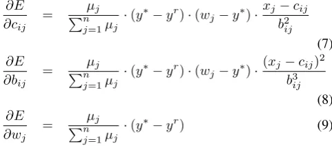
Gaussian membership function is used as the membership function, the following relation holds.

∂E ∂cij =

µj

∑n j=1µj

·(y∗−yr)·(wj−y∗)·xj−cij b2

ij

(7)

∂E ∂bij =

µj

∑n j=1µj

·(y∗−yr)·(wj−y∗)·(xj−cij) 2

b3 ij

(8)

∂E

∂wj =

µj

∑n j=1µj

·(y∗−yr) (9)

The conventional learning algorithm is shown as Fig.1 [1]– [3], where θ and Tmax are threshold and the maximum

number of learning, respectively. Note that the method is generative one. The method is called learning algorithm A.

B. Neural gas and K-means methods

Vector quantization techniques encode a data space, e.g., a subspaceV⊆Rm, utilizing only a finite setC={ci|i∈Zr}

of reference vectors (also called cluster centers), where m

andrare positive integers.

Let the winner vectorci(v)be defined for any vectorv∈V

as follows:

i(v) = arg min i∈Zr

||v−ci|| (10)

'ŝǀĞŶߝ௜௡௧ǡ ߝ௙௜௡ǡ ܶ௠௔௫͘>Ğƚݐ ൌ ͳ͘

ĂĐŚƌĞĨĞƌĞŶĐĞǀĞĐƚŽƌࢉ௜

ŝƐƐĞůĞĐƚĞĚƌĂŶĚŽŵůLJ͘

'ŝǀĞŶ࢜ א ࢂ ǁŝƚŚ݌ ࢜ ͘ ĞƚĞƌŵŝŶĞƚŚĞŶĞŝŐŚďŽƌŚŽŽĚͲ

ƌĂŶŬŝŶŐ݇௜ ࢜ǡ ࢉ௜ ĨŽƌ݅ א ܼ௥͘

hƉĚĂƚĞࢉ௜ĨŽƌ݅ א ܼ௥

ƵƐŝŶŐƋ͘;ϭϰͿĂŶĚ ߝ௜௡௧՚ ߝ௜௡௧ ߝ௜௡௧Ȁߝ௙௜௡ ௧Ȁ்೘ೌೣ

ݐ ൌ ܶ௠௔௫͘

E ݐ ՚ ݐ ൅ ͳ

[image:2.595.50.291.507.613.2]

zĞƐ EŽ

Fig. 2. Neural Gas method

From the finite setS,V is portioned as follows:

Vi={v∈V|||v−ci||≤||v−cj||f or j∈Zr} (11)

The evaluation function for the partition is defined as follows:

E= r

∑

i=1

∑

v∈Vi

||v−ci(v)||2 (12)

For neural gas method [14], the following method is used: Given an input data vector v, we determine the neighborhood-rankingcik for k∈Zr∗−1, being the reference

vector for which there arek vectorscj with

||v−cj||<||v−cik|| (13) If we denote the numberkassociated with each vectorci

byki(v,ci), then the adaption step for adjusting theci’s is

given by

△ci = ε·hλ(ki(v,c))·(v−ci) (14) hλ(ki(v,c)) = exp(−ki(v,c)/λ) (15)

where ε∈[0,1] and λ > 0. The number λ is called decay constant.

If λ→0, Eq.(14) becomes equivalent to the K-means method [14]. Otherwise, not only the winner ci0 but the

second, third nearest reference vectorci1,ci2, etc., are also

updated.

Let p(v) be the probability distribution of data vectors for

V. The flowchart of the conventional neural gas algorithm is shown as Fig.2 [14], where εint, εf in, θ and Tmax are learning constants, threshold and the maximum number of learning, respectively. The method is called learning algo-rithm NG.

based on p(v)is given [14].

By using Learning Algorithm NG, learning method of fuzzy systems is shown as follows [13] : In this case, assume that the distribution of learning data D∗ is discrete uniform one. Let n0 be the initial number of rules.

Learning Algorithm B

Step B1 : For learning data D∗, Learning Algorithm NG is performed by usingD∗ as the setV. As a result, the set

cof inference vectors forD∗ is made, where|c|=n0.

Step B2 : Each initial valuecij is set to a reference vector. Let

bij= 1 mi

∑

xk∈Ci

(cij−xkj)2, (16)

where Ci and mi are set of element and the number of learning data belonging to the i-th cluster Ci. Each initial weightwiis selected randomly. Further, Step A1 of Learning Algorithm A is performed.

Step B3 : The Steps A3 to A9 of learning algorithm A are performed.

C. Determination of weights using the generalized inverse method

Let us explain fuzzy inference systems and interpolation problem using the generalized inverse method [3]. This problem can be stated mathematically as follows:

Given P points{xp _{= (x}p

1,· · ·, xpm)|p∈ZP} and P real

numbers {yr_p|p∈Z

P}, find a function f :Rm→R such that

the following conditions are satisfied :

f(xp) =y_pr p∈ZP (17) In the case of fuzzy inference system, this problem is solved as follows:

yp=f(xp) = n

∑

i=1

wiϕpi(||xp−ci||) (18) ϕpi(||xp−ci||) =

µi

∑n i=1µi

(19)

That is,

Φw=y, (20)

where

Φ =

     

ϕ11 ϕ12 · · · ϕ1n

ϕ21 ϕ22 · · · ...

..

. ... . .. ...

ϕP1 ϕP2 · · · ϕP n

    

 (21)

Let P = n and xi _{= c}

i. The width parameters are

determined by Eq.(19). Then, ifϕi(·)is suitably selected as Gaussian function, then the solution of weights w is obtained as

w= Φ−1y (22) Let us consider the casen < P. This is the realistic case. The optimal solution w∗ that minimizes E=||yr_−Φw||2

can be obtained as follows :

w+= ΦTyandEmin =||(I−Ψ)y||2, (23)

whereΦ+_≜[ΦT_Φ]−1_ΦT_,Ψ≜ΦΦT _{and I is identify matrix}

ofP×P.

Φ+ _{is called the generalized inverse of Φ. The method}

usingΦ+ _{to determine the weights is called the generalized}

inverse method (GIM) [3].

D. The appearance frequency of input data based on the rate of change of output

Learning Algorithm B is a method that determines the initial assignment of fuzzy rules by vector quantization using the setD∗of input for learning data. In this case, the set of output in learning dataDis not used to determine the initial assignment of fuzzy rules. In the previous paper, Kishida proposed a method considering both input and output data to determine the initial assignment of fuzzy rules [12].

Based on the literature [12], the appearance frequency is defined as follows : LetD andD∗ be the sets of learning data defined in 2.1.

Calculation Algorithm for the appearance frequency Step 1 : Give an input data xi∈D∗, we determine the neighborhood-ranking (xi0_,xi1_,· · ·_,xik_,· · ·_,xiP−1_{) of the}

vector xi _{with x}i0 _{= x}i_{, x}i1 _{being closest to x}i _and

xik_{(k = 0,}· · ·_{, P} −_{1) being the vector x}i _{for which there} arek vectorsxj _with||xi_−xj_||<||xi_−xik||_.

Step 2 :DetermineH(xi_{)which shows the degree of change}

of inclination of the output around output data to input data

xi, by the following equation:

H(xi) = M

∑

l=1

yi_−yil

||xi−_xil||

, (24)

where xil _{for l}∈_Z

M means the l-th neighborhood-ranking

ofxi_,i∈Z

P andyi andyil are output for inputxi andxil,

respectively. The number M means the range considering

H(x).

Step 3 :Determine the appearance frequencypM(xi_)forxi

by normalizingH(xi_).

pM(xi) = H(x i₎

∑P

j=1H(xj)

(25)

Learning algorithm C using the appearance frequency is shown as follow [12]:

Learning Algorithm C

Step 1 : θ,T_max0 ,Tmax,nandM0for1≤M0are set. Initial

value ofcij,bij andwi are set randomly. LetM←M0. The

appearance frequencypM(xi)for xi∈D∗ is computed. Step 2 : Select a data (xp_{, y}p_{) based on p}

M(xp, yp) for 1≤p≤P.

Step 3 : Updatecij by Eq.(14).

Step 4 : Ift < T0

max, go to Step 2 witht←t+ 1, otherwise

go to Step 5 witht←1.

Step 5 : Determinebij by Eq.(16). Step 6 : Letp←1.

Step 7 : Given a data(xp_{, y}r p)∈D.

Step 8 : Calculate µi andy∗ by Eqs.(2) and (4).

Step 9 : Update parameterscij,bij andwij by Eqs.(7), (8) and (9).

Step 10 : Ifp < P then go to Step 7 withp←p+ 1. Step 11 : If E > θ andt < Tmax then go to Step 7 with

t←t+ 1, where E is computed as Eq.(5), and if E < θ

n←n+1and initial value ofcij,bijandwiare set randomly, M←M0 and the appearance frequencypM(xi)for xi∈D∗

is computed.

III. THE PROPOSED METHOD

It is shown that learning method C using VQ and SDM is effective in accuracy and the number of rules to other methods. However, it needs a great deal of learning time. The cause could be that both of VQ and SDM are local search methods. On the other hand, it has been shown that a learning method of RBF networks using VQ and GIM is much fast compared to other learning methods [3]. Specifically, the method using GIM seems to be effective compared to methods using SDM, because the method is not local search. However, the method using only VQ and GIM is not always effective [15]. Therefore, we propose a new learning method composed of three stages using VQ, GIM and SDM. The three stages are iterated in the outer loop of the algorithm. The first stage adjusts the center and width parameters by using VQ, the second one updates the weight parameters by using GIM, and the last one adjusts all three parameters by using SDM. With iterating processes, parameters of the result of SDM are set to ones of the next process if the inference error is improved.

The proposed method is shown as follows: Learning Algorithm E

Step 1 : θ, T0

max, Tmax, M0, Mmax andβ for 1≤Mmax

andβ < P are set. LetM←M0. Initial values ofcbestij ,bbestij

andw_ibestare set randomly. LetEbestbe the MSE for fuzzy inference system with cbest_ij ,bbest_ij andwbest_i . Letn←n0.

(Stage 1: Learning by VQ)

Step 2 : Letcij←cbestij ,bij←bbestij ,wi←wibest andt= 1.

Step 3 : Select a data (xp_{, y}p_{) based on p}

M(xp, yp) for 1≤p≤P.

Step 4 : Updatecij by Eq.(14).

Step 5 : Ift < T0

max, go to Step 3 witht←t+ 1, otherwise

go to Step 6 with t←1.

Step 6 : Determinebij by Eq.(16). (Stage 2: Learning by GIM) Step 7 : Determinewi by Eq.(23). (Stage 3: Learning by SDM) Step 8 : Letp←1.

Step 9 : Given a data(xp, y_pr)∈D.

Step 10 : Calculate µi andy∗ by Eqs.(2) and (4).

Step 11 : Update parameters cij, bij and wij by Eqs.(7), (8) and (9).

Step 12 : Ifp < P then go to Step 8 withp←p+ 1. Step 13 : IfE(t)> θandt < Tmaxthen go to Step 9 with t←t+ 1, whereE is computed as Eq.(5).

Step 14 : If E(t) < Ebest then cbestij ←cij, bbestij ←bij, wbest

i ←wi andEbest←E(t).

Step 15 : If E(t) > θ and M < Mmax then go to Step 2 with M←M +β, else if E(t) < θ, then the algorithm terminates, otherwise go to Step 2 withn←n+ 1,M←M0

andcbest_ij ,bbest_ij andw_ibest are set randomly.

In order to compare the proposed method with conven-tional ones, the following methods are used (See Fig.3): (A) Method A is one based on the algorithm of Fig.1 [1], [2]. Initial parameters ofc,bandware set randomly and all

^ĞůĞĐƚc͕b ĂŶĚw ƌĂŶĚŽŵůLJ͘

ĞƚĞƌŵŝŶĞƉĂƌĂŵĞƚĞƌƐ c ĂŶĚb ďLJE'͘

ĞƚĞƌŵŝŶĞƉĂƌĂŵĞƚĞƌƐ c ĂŶĚb ďLJE'͘

ĞƚĞƌŵŝŶĞ ƉĂƌĂŵĞƚĞƌƐc ĂŶĚb ďLJE'͘ >ĞĂƌŶŝŶŐĚĂƚĂ

௣_ǡ ௣௥ȁ א ௉

>ĞĂƌŶŝŶŐĚĂƚĂ ௣_ǡ

௣௥ȁ א ௉

>ĞĂƌŶŝŶŐĚĂƚĂ ௣_{ȁ א}

௉

hƉĚĂƚĞc, b ĂŶĚw ďLJ^D͘

hƉĚĂƚĞc, b ĂŶĚw ďLJ^D͘

hƉĚĂƚĞc, b ĂŶĚw ďLJ^D͘

hƉĚĂƚĞc, b ĂŶĚw ďLJ^D͘ hƉĚĂƚĞw

ďLJŵĂƚƌŝdž ĐŽŵƉƵƚĂƚŝŽŶ͘

;Ϳ

;Ϳ

;Ϳ

;Ϳ

;Ϳ

ĞƚĞƌŵŝŶĞƉĂƌĂŵĞƚĞƌƐ c ĂŶĚb ďLJE'͘ >ĞĂƌŶŝŶŐĚĂƚĂ

௣_ǡ ௣௥ȁ א ௉

hƉĚĂƚĞc, b ĂŶĚw ďLJ^D͘ ^ĞůĞĐƚw

ƌĂŶĚŽŵůLJ͘

^ĞůĞĐƚw ƌĂŶĚŽŵůLJ͘

^Ğƚw ƚŽ ƚŚĞƌĞƐƵůƚ ŽĨכଵ_͘

Fig. 3. Concept of conventional and proposed algorithms, where SDM and NG mean Steepest Descent Method and Neural Gas method, and the mark ∗1means that initial values ofware selected randomly.

parameters are updated using SDM until the inference error become sufficiently small.

(B) Method B is known as learning method of RBF networks [3], [9], [13]. Initial values ofcare determined usingD∗by VQ andbis computed by Eq.(16). Weight parametersware randomly selected. Further, all parameters are updated using SDM until the inference error become sufficiently small. (C) Method C is proposed in Ref. [9]. Initial values of

c are determined using D by VQ and b is computed by Eq.(16). Weight parameters are randomly selected. Further, all parameters are updated using SDM until the inference error become sufficiently small.

Note that the difference between Methods B and C is that learning dataD orD∗ is used in algorithm.

(D) Method D is proposed in Ref. [17]. It is learning method composed of iterating two stages. The center parameters

c are determined using D by VQ and b is computed by Eq.(16). Weight parametersw is set to the results of SDM, where the initial values of w are set randomly. Further, all parameters are updated using SDM for the definite number of learning time. With iterating processes, parameters of the result of SDM are set to ones of the next process. Outer iterating process is repeated until the inference error become sufficiently small.

(E) Method E is the proposed one. It is learning method composed of iterating three stages. It starts by breaking the method into three stages: learning in the first stage, inter-mediate stage of adjusting the center and width parameters, and the next stage of updating the weight parameters using GIM. As for the final stage, three parameters are updated using SDM for the definite number of learning time. With iterating processes, parameters of the result of SDM are set to ones of the next process.

IV. NUMERICAL SIMULATIONS

In order to show the effectiveness of Learning Algorithm E, simulations of function approximation and classification problems are performed.

A. Performance of initial assignment of parameters

[image:4.595.316.537.55.223.2]

TABLE I

CONDITIONS OFALGORITHMS FOR NUMERICAL SIMULATION OF FUNCTION APPROXIMATION

A B C D E

Kcij 0.01 0.01 0.01 0.01 0.01

Kbij 0.01 0.01 0.01 0.01 0.01

Kwi 0.1 0.1 0.1 0.1 0.1

εinit

0.1 0.1 0.1 0.1

εf in

0.01 0.01 0.01 0.01

λ

0.7 0.7 0.7 0.7

TABLE II

THE RESULTS FOR FUNCTION APPROXIMATION MSE for Learning(×10−4_{) 0.10}

A MSE of Test(×10−4_{) 1.63}

t 438.1

MSE of Learning(×10−4_{) 0.10}

B MSE of Test(×10−4_{) 1.86}

t 106.7

MSE of Learning(×10−4_{) 0.10}

E MSE of Test(×10−4_{) 2.04}

t 90.3

that the method E without outer iterating process and with iterating process of SDM until the inference error becomes sufficiently small.

The system is identified by fuzzy inference systems. This simulation uses four systems specified by the following functions with 4-dimensional input space [0,1]4_{, and one}

output with the range[0,1]:

y = (2x1+ 4x 2 2+ 0.1)2 37.21

×(4 sin(πx3) + 2 cos(πx4) + 6)

12 (26)

The numbersM,M0,β,Mmaxand the number of rulesn

are 200, 200, 0, 200 and 20, respectively. The thresholdθis

1.0×10−4_{. Note that the number of rules is fixed. The results}

are average from ten trials. The results show that appropriate initial assignment of parameters results in a fast learning method.

B. Function approximation problems

In order to show the effectiveness of Learning Algo-rithm E, numerical simulations of function approximation are performed. The systems are identified by fuzzy infer-ence systems. This simulation uses four systems specified by the following functions with 4-dimensional input space

[0,1]4_{(Eqs.(27) and (28)) and [−1,1]}4_{((29) and (30)), and}

one output with the range[0,1];

y = (2x1+ 4x 2 2+ 0.1)

2

37.21

×(4 sin(πx3) + 2 cos(πx4) + 6)

12 (27)

y = (sin(2πx1)×cos(x2)×sin(πx3)×x4+ 1.0) 2.0

(28)

y = (2x1+ 4x 2 2+ 0.1)2 74.42

+(3e

3x3_{+ 2e}−4x4₎−0.5−_0.077

4.68 (29)

TABLE III

CONDITIONS OFALGORITHMS FOR NUMERICAL SIMULATION OF FUNCTION APPROXIMATION PROBLEMS

A B C D E

Tmax 50000 50000 50000 5000 50

Kcij 0.01 0.01 0.01 0.01 0.01

Kbij 0.01 0.01 0.01 0.01 0.01

Kwi 0.1 0.1 0.1 0.1 0.1

εinit

0.1 0.1 0.1 0.1

εf in

0.01 0.01 0.01 0.01

λ

0.7 0.7 0.7 0.7

TABLE IV

INITIAL PARAMETERS OF NUMERICAL SIMULATION FOR FUNCTION APPROXIMATION PROBLEMS OFEQS.(27), (28), (29)AND(30)

θ 1.0×10−4

M 200

M0 200

β 50

Mmax 400

♯Learning data 512 ♯Test data 6400

y = (2x1+ 4x 2 2+ 0.1)2 74.42

+(4 sin(πx3) + 2 cos(πx4) + 6)

446.52 (30)

Tables III and IV show the initial conditions for sim-ulations. In Table III, A, B, C, D and E mean Learning Algorithms A, B, C, D and E. Table V shows the results for simulations. In Table V, the number of rules, MSE’s for learning and test, and learning time(second) are shown, where the number of rules means one when the threshold

θ= 1.0×10−4_{of inference error is achieved in learning. The}

result of simulation is the average value from twenty trials. As a result, the proposed method E reduces the learning time to about one-tenth compared to other methods.

C. Classification problems

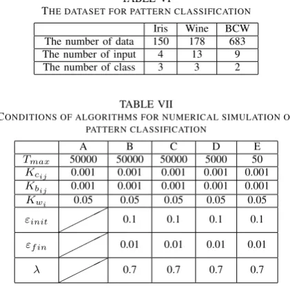
Iris, Wine and BCW data from UCI database shown in Table VI are used for numerical simulation [16]. In this

TABLE V

THE RESULTS FOR FUNCTION APPROXIMATION PROBLEMS Eq(27) Eq(28) Eq(29) Eq(30) The number of rules 4.2 13.6 7.2 5.1 A MSE Learning 0.40 0.71 0.43 0.28

(×10−4) Test 0.52 1.09 1.00 0.49 Learning time (s) 254.9 2617.5 777.9 365.7 The number of rules 5.6 14.9 5.2 3.7 B MSE Learning 0.18 0.77 0.49 0.33

(×10−4) Test 0.27 1.42 1.11 0.48 Learning time (s) 624.5 6766.1 513.0 255.5 The number of rules 4.8 15.6 5.5 4.0 C MSE Learning 0.21 0.72 0.54 0.88

(×10−4) Test 0.34 1.33 0.69 0.53 Learning time (s) 350.2 3125.0 447.6 210.0 The number of rules 3.0 8.4 4.0 3.0 D MSE Learning 0.28 0.69 0.66 0.21

(×10−4) Test 0.35 1.25 0.76 0.23 Learning time (s) 268.5 1673.3 425.9 267.0 The number of rules 3.0 8.0 8.6 5.5 E MSE Learning 0.30 0.88 0.84 0.75

[image:6.595.63.274.57.271.2]

TABLE VI

THE DATASET FOR PATTERN CLASSIFICATION Iris Wine BCW The number of data 150 178 683 The number of input 4 13 9 The number of class 3 3 2

TABLE VII

CONDITIONS OF ALGORITHMS FOR NUMERICAL SIMULATION OF PATTERN CLASSIFICATION

A B C D E

Tmax 50000 50000 50000 5000 50

Kcij 0.001 0.001 0.001 0.001 0.001

Kbij 0.001 0.001 0.001 0.001 0.001

Kwi 0.05 0.05 0.05 0.05 0.05

εinit

0.1 0.1 0.1 0.1

εf in

0.01 0.01 0.01 0.01

λ

0.7 0.7 0.7 0.7

simulation, 5-fold cross-validation is used. Tables VII and VIII show the initial conditions for simulations and Table IX shows the result of classification for each algorithm. In Table IX, the number of rules, RM’s for learning and test, and learning time(second) are shown, where RM means the rate of misclassification. It is shown that the proposed method E is realized with high accuracy in a short time compared with other methods.

V. CONCLUSION

In this paper, we proposed a new learning method com-posed of iterating three stages. It started by breaking the method into three stages: learning in the first stage, inter-mediate stage adjusting the center and width parameters, and the next stage of updating the weight parameters using the generalized inverse method (GIM). As the final stage, three parameters were updated by learning based on SDM. In order to demonstrate the effectiveness of the proposed method, numerical simulations for function approximation and pattern classification problems were performed. It was shown that the proposed method reduces the learning time to about one-tenth compared to other methods in function approximation and is realized with high accuracy in a short time compared with other methods in classification problem. In the future work, we will propose faster learning algo-rithm using VQ and the generalized inverse method com-pared to other methods.

REFERENCES

[1] B. Kosko, Neural Networks and Fuzzy Systems, A Dynamical Systems Approach to Machine Intelligence, Prentice Hall, Englewood Cliffs, NJ, 1992.

[2] C. Lin and C. Lee, Neural Fuzzy Systems, Prentice Hall, PTR, 1996. [3] M.M. Gupta, L. Jin and N. Homma, Static and Dynamic Neural

Networks, IEEE Press, 2003.

[4] J. Casillas, O. Cordon, F. Herrera and L. Magdalena, Accuracy Improvements in Linguistic Fuzzy Modeling, Studies in Fuzziness and Soft Computing, Vol. 129, Springer, 2003.

[5] B. Liu, Theory and Practice of Uncertain Programming, Studies in Fuzziness and Soft Computing, Vol. 239, Springer, 2009.

[6] S. M. Zhoua and J. Q. Ganb, Low-level interpretability and high-level interpretability: a unified view of data-driven interpretable fuzzy system modeling, Fuzzy Sets and Systems 159, pp.3091-3131, 2008.

TABLE VIII

INITIAL PARAMETERS FOR NUMERICAL SIMULATION OF PATTERN CLASSIFICATION

Iris Wine BCW

θ 1.0×10−2 _1.0×10−2 _2.0×10−2

M 100 100 200 M0 30 40 200

β 10 10 30

Mmax 120 130 470

TABLE IX

THE RESULT FOR PATTERN CLASSIFICATION Iris Wine BCW the number of rules 3.4 7.8 14.4 A RM for Learning(%) 3.0 1.4 1.6

RM of Test(%) 3.3 10.3 4.3 learning time(s) 40.4 613.1 9161.4 the number of rules 2.0 20.8 26.0 B RM of Learning(%) 3.3 13.6 2.2

RM of Test(%) 3.3 16.6 3.5 learning time(s) 16.8 7.4 9.6 the number of rules 3.4 7.4 9.6 C RM of Learning(%) 2.8 2.1 2.0 RM of Test(%) 4.7 5.1 4.6 learning time(s) 38.9 529.0 2763.4 the number of rules 2.0 3.2 4.8 D RM of Learning(%) 3.3 1.5 1.6 RM of Test(%) 4.0 6.7 3.8 learning time(s) 25.1 204.8 1648.7 the number of rules 3.7 2.5 2.5 E RM of Learning(%) 3.3 1.1 1.3 RM of Test(%) 3.8 6.5 2.1 learning time(s) 8.6 3.3 37

[7] S. Fukumoto, H. Miyajima, K. Kishida and Y. Nagasawa, A Destruc-tive Learning Method of Fuzzy Inference Rules, Proc. of IEEE on Fuzzy Systems, pp.687-694, 1995.

[8] O. Cordon, A historical review of evolutionary learning methods for Mamdani-type fuzzy rule-based systems, Designing interpretable genetic fuzzy systems, Journal of Approximate Reasoning, 52, pp.894-913, 2011.

[9] K. Kishida, H. Miyajima, M. Maeda and S. Murashima, A Self-tuning Method of Fuzzy Modeling using Vector Quantization, Proceedings of FUZZ-IEEE’97, pp397-402, 1997.

[10] N. Yubazaki, J. Yi and K. Hirota, SIRMS(Single Input Rule Mod-ules) Connected Fuzzy Inference Model, J. Advanced Computational Intelligence, 1, 1, pp.23-30, 1997.

[11] H. Miyajima, N. Shigei and H. Miyajima, Fuzzy Inference Systems Composed of Double-Input Rule Modules for Obstacle Avoidance Problems, IAENG International Journal of Computer Science, Vol. 41, Issue 4, pp.222-230, 2014.

[12] K. Kishida and H. Miyajima, A Learning Method of Fuzzy Inference Rules using Vector Quantization, Proc. of the Int. Conf. on Artificial Neural Networks, Vol.2, pp.827-832, 1998.

[13] S. Fukumoto, H. Miyajima, N. Shigei and K. Uchikoba, Decision Procedure of the Initial Values of Fuzzy Inference System Using Counterpropagation Networks, Journal of Signal Processing, Vol.9, No.4, pp.335-342, 2005.

[14] T. M. Martinetz, S. G. Berkovich and K. J. Schulten, Neural Gas Network for Vector Quantization and its Application to Time-series Prediction, IEEE Trans. Neural Network, 4, 4, pp.558-569, 1993. [15] W. Pedrycz, H. Izakian, Cluster-Centric Fuzzy Modeling, IEEE Trans.

on Fuzzy Systems, Vol. 22, Issue 6, pp. 1585-1597, 2014.

[16] UCI Repository of Machine Learning Databases and Domain Theories, ftp://ftp.ics.uci.edu/pub/machinelearning-Databases.