Abstract—This study provides analytical modeling of
condition monitoring with periodic imperfect inspections of a stochastically deteriorating system. An inspection consists of checking the system state parameter against the critical threshold level in the upcoming time intervals. A new decision rule is proposed for inspecting the system condition, which is based on the comparison of the time of inspection with the estimated remainder of the time to failure. Based on this decision rule, general expressions are derived for calculating the probabilities of correct and incorrect decisions. The proposed approach is illustrated by deriving the probabilities of correct and incorrect decisions for a linear stochastic deterioration process model. Based on the derived expressions, the Bayes risk and minimum total error probability criteria are specified to determine the optimal threshold. A numerical example is given to illustrate the proposed approach for determining the optimal threshold when checking system suitability.
Index Terms—Decision rule, functional failure level,
imperfect inspection, measurement error of time to failure, threshold
I. INTRODUCTION
URRENTLY, condition-based maintenance (CBM) is
considered to be a perspective approach to improve the operational reliability and reduce the operating costs of several military and civil engineering systems. The basic maintenance operation of this type is condition monitoring, which can be continuous or periodic. Continuous monitoring is impractical in some cases. It can be more practical to monitor the system periodically, for example, due to the cost reasons. Evidently, condition monitoring is preferred among other maintenance techniques in those cases where system deterioration can be measured, and wherein the system enters the failed state when the state parameter deteriorates beyond the level of functional failure. Over the past 10–15 years, many CBM models have been developed [1]-[5]. Among the existing CBM models, there are almost no models considering the probabilities of correct and incorrect decisions when inspecting the system condition. However, the condition monitoring data are always affected to some degree by measurement errors and noise, which may cause incorrect decisions. Some of the published models include measurement error, but they do not contain expressions to calculate the probabilities of
Manuscript received March 01, 2015; revised March 28, 2015. A. Raza is with the Department of the President’s Affairs, Overseas Projects & Maintenance, Abu Dhabi, UAE (e-mail: ahmed.awan786@ gmail.com).
V. Ulansky is with the Electronics Department, National Aviation University, Kiev, 03058 Ukraine (00380632754982; e-mail: [email protected]).
incorrect decisions. The inspection model considered in [6] includes the original deterioration process along with a normally distributed measurement error. Based on this model, a decision rule is analyzed, and optimal monitoring policies are found. The same approach is used in [7] to include measurement error in a Wiener diffusion process-based degradation model. A similar approach is used in [8] to determine the likelihood function for more than one inspection. The authors propose a simple extension to the Bayesian updating model such that the model can incorporate the results of inaccurate measurements. In [9], the proposed degradation model uses a random effects Wiener process with measurement errors. A filtering algorithm is developed to estimate the joint distribution of the degradation rate and the current degradation levels. The traditional Wiener process with positive drifts compounded with Gaussian noises is investigated in [10]. A mixed effects model with measurement errors is developed. The model includes several existing Wiener processes as its limiting cases. In [11], a continuously degrading system that is being monitored at regular time intervals is considered assuming that maintenance is imperfect, and the system deteriorates according to a gamma process. An optimal threshold to perform maintenance and an optimal time interval for monitoring the system are determined. In [12], a model is considered under assumptions that the maintenance is imperfect and the degradation is a continuous-time Markov process. A proposed strategy combines both inspection and continuous monitoring to reduce unnecessary inspection and improve the system’s reliability. In [13], the research work is focused on imperfect inspection policy investigation when not all defects are identified during inspection action performance, and the probability of defect identification is not a constant variable. The two basic cases of imperfect inspection are analyzed. In the first case, the probability of defect detecting during inspection is constant. In the second case, this probability is increasing linearly according to the defect symptoms visibility increase. In [14], CBM policies with imperfect operability checks are considered. The proposed expressions for probabilities of correct and incorrect decisions depend on the deterioration process parameters and uncertainty errors.
This paper presents a more general condition monitoring model with imperfect inspections, which assumes that the monitoring data are mixed with measurement errors or noise and that incorrect decisions can occur when checking the system suitability in the coming interval of operation. The probabilities of correct and incorrect decisions are determined based on such a concept as measurement error of time to failure.
A Probabilistic Model of Periodic Condition
Monitoring with Imperfect Inspections
Ahmed Raza and Vladimir Ulansky
II. DECISION RULE AND SPACE OF EVENTS
In this study, a deteriorating system subjected to random failure is considered. It is assumed that the state of a system is completely identified by the value of one parameter X(t), which is a nonstationary stochastic process with continuous time. A system should be inspected at successive times tk (k
= 1, 2, …), where t0 = 0. When the system state parameter exceeds its functional failure level FF, the system passes into the failed state. In the presence of measurement error in the inspection of the system state parameter, let Z(tk) be the
measured value of X(tk) and relate to X(tk) by the following
equation:
tk X tk Y tkZ , (1) where Y(tk) is the measurement error of the system state
parameter at time tk.
We introduce the following decision rule when inspecting the system condition at time tk. If z(tk) < PF, the system is
said to be suitable over the interval (tk, tk+1), where PF (PF < FF) is the critical threshold level equivalent to the potential failure level of the system state parameter X(t). If z(tk) ≥ PF,
the system is said to be unsuitable, and it should not be used in the interval (tk, tk+1). Thus, this decision rule is aimed
toward the rejection of systems that are unsuitable for use in the next operation interval.
From the perspective of the system suitability for use in the interval (tk, tk+1) when checking the parameter X(t) at
time t = tk , one of the following mutually exclusive events
may appear:
, ,
, ,
, ,
, ,
, ,
, ,
1 6
1 5
1 1
4
1 1
3
1 1
2
1 1
1
PF t Z FF t X t t H
PF t Z FF t X t t H
PF t Z FF t
X FF t X t t H
PF t Z FF t
X FF t X t t H
PF t Z FF t
X t t H
PF t Z FF t
X t t H
k k
k k
k k
k k
k k
k k
k
k k
k k
k
k k
k k
k k
k k
(2)
where H1(tk, tk+1) is the joint occurrence of two events: the
system is suitable for use over the interval (tk, tk+1) and
judged to be suitable when checking at time point tk; H2(tk, tk+1) is the joint occurrence of two events: the system is
suitable for use over the interval (tk, tk+1) and judged as
unsuitable when checking at time tk; H3(tk, tk+1) is the joint
occurrence of the following events: the system is operable at time tk but fails up to time tk+1; when checking the system at
time tk, it is judged as suitable for using in the interval (tk, tk+1); H4(tk, tk+1) is the joint occurrence of the following
events: the system is operable at time tk but fails up to time tk+1; when checking the system at time tk, it is judged as
unsuitable for using in the interval (tk, tk+1); H5(tk, tk+1) is the
joint occurrence of the following events: at time point tk, the
system is inoperable and judged as suitable for using over the interval (tk, tk+1); and H6(tk, tk+1) is the joint occurrence of
the following events: at time point tk, the system is
inoperable and judged as unsuitable for using over the interval (tk, tk+1).
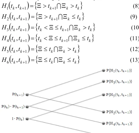
The graph of decision making when checking system suitability at time tk is shown in Fig. 1. As seen from the
graph in Fig. 1, the system a priori can be in one of the three
states: state of suitability with probability P(tk+1), operable
but not suitable state with probability P(tk) − P(tk+1), and
inoperable state with probability 1 − P(tk), where P(t) is the
system reliability function.
Let us find the probabilities of events (2). Assume that a random variable Ξ (Ξ ≥ 0) denotes the failure time of a system with failure density function ω(ξ). We introduce two new random variables associated with the critical threshold level PF. Let Ξ0 denote a random time of a system
operation until it exceeds the critical threshold level PF by the parameter X(t), and let Ξk denote a random assessment
of Ξ0 based on inspection results at time tk.
The random variables Ξ, Ξ0, and Ξk are determined as the
smallest roots of the following stochastic equations:
t FF0X (3)
t PF0X (4)
t PF 0Z k (5) From the definition of the random variable Ξk, it follows
that
PF t Z t
k PF t
Z t
k k
k k k
if ,
... , 2 , 1 if
,
(6) Based on (6), the previously introduced decision rule can be converted to the following form: the system is judged to be suitable at time point tk if ξk > tk; otherwise (i.e., if ξk ≤ tk), the system is judged to be unsuitable, where ξk is the
realization of Ξk for the system under inspection.
From (5), it follows that Ξk is a function of random
variables Ξand Y(tk). The presence of Y(tk) in (5) leads to a
random measurement errorwith respect to time to failure at time tk, which is defined as follows:
... , 2 , 1
,
k k k (7) The additive relationship between random variables Ξ (0 < Ξ < ∞) and Λk (−∞ < Λk < ∞) leads to −∞ < Ξk < ∞.
Mismatch between the solutions of (3) and (5) results in the appearance of one of the following mutually exclusive events when inspecting system suitability at time tk:
tk tk
tk k tk
H1 , 1 1 (8)
tk tk
tk k tk
H2 , 1 1 (9)
tk tk
tk tk k tk
H3 , 1 1 (10)
tk tk
tk tk k tk
H4 , 1 1 (11)
tk tk
tk k tk
H5 , 1 (12)
tk tk
tk k tk
[image:2.595.304.545.529.758.2]H6 , 1 (13)
Fig. 1. Graph of decision making when checking system suitability at time
From (10) and (11), we see that in terms of system suitability over the interval (tk, tk+1), the event H3(tk)
corresponds to the incorrect decision, and the event H4(tk)
corresponds to the correct decision. When the event H3(tk)
occurs, the unsuitable system is incorrectly allowed to be used over the time interval (tk, tk+1). From the viewpoint of
system operability checking, the event H3(tk) corresponds to
the correct decision, and the event H4(tk) corresponds to the
incorrect decision.
The event H2(tk) is further called a “false failure,” and
events H3(tk) and H5(tk) are called “undetected failure 1” and
“undetected failure 2,” respectively. Events H1(tk), H4(tk),
and H6(tk) correspond to the correct decisions pertaining to
system suitability and unsuitability.
Note that even when Y(tk) = 0 (k = 1, 2, …), incorrect
decisions are possible when checking system suitability. In fact, if Y(tk) = 0, expressions (8)−(13) are converted to the
following form:
tk tk
tk tk
H1 , 1 1 0 , (14)
tk tk
tk tk
H2 , 1 1 0 , (15)
tk tk
tk tk tk
H3 , 1 1 0 , (16)
tk tk
tk tk tk
H4 , 1 1 0 , (17)
1
5 tk,tk
H Ø, (18)
tk tk
tk tk
H6 , 1 0 , (19) where Ø denotes the impossible event.
The errors arising at Y (tk) = 0 are methodological in
nature and nonremovable with the decision rule used herein. III. PROBABILITIES OF CORRECT AND INCORRECT
DECISIONS
Determination of probabilities (8)−(13) is based on the use of the well-known formula for calculating the probability of hitting a random point {Ξ, Ξk} to the known
area. Denoting the joint probability density function (PDF) of random variables {Ξ, Ξk} as ω0(ξ, ξk), it is easy to
determine that
H t t
u
du d
P k
t t k
k k
k k
1
,
, 1 0
1 (20)
H t t
u
du d
P k
t t
k k
k
k k
1
,
, 1 0
2 (21)
H t t
u
du d
P t k
t t k
k k
k
k k
1
,
, 1 0
3 (22)
H t t
u
du d
P t k
t t
k k
k
k
k k
1
,
, 1 0
4 (23)
H t t
u
du d
P t k
t k
k k
k
k
0 0 1
5 , , (24)
H t t
u
du d
P k k t t
k k k k
0 0 1
6 , , (25)
As seen from (20)−(25), to determine the probabilities of correct and incorrect decisions, we need to know the joint PDF ω0(ξ, ξk). We denote the conditional PDF of random
variable Λk as f0(λk|ξ) under the condition that Ξ = ξ. The
following statement allows us to express PDF ω0(ξ, ξk)
using PDFs ω(ξ) and f0(λk|ξ).
Theorem 1. The following formula holds for the joint PDF of random variables Ξ and Ξk:
ξ,ξ
ωξ
ξ ξξ
ω0 k f0 k (26)
Proof. Using the multiplication theorem of the PDFs, we can write
ξ,ξ
ω ξ ω
ξ ξω0 k 1 k , (27) where ω1(ξk|ξ) is the conditional PDF of random variable
Ξk under the condition that Ξ = ξ. When Ξ = ξ, random
variable Ξk can be represented as Ξk= ξ + Λk. By virtue of
the additive relationship between random variables Ξ and Λk,the following equality holds:
ξ ξ ξ ξξ
ω1 k f0 k (28) Substituting (28) in (27), we obtain (26).
The substitution of (26) to (20) gives
H t t
f
u
du d
P k
t t k
k k
k k
1
0 1
1 , (29)
Assuming that gk = uk − ϑ in (29), we have
f g dg d
t t H
P k
t t k
k k
k k
1
0 1
1 , (30)
Carrying out a similar change of variables in (21)−(25), we obtain
H t t
f
g
dg d
P k
t
t
k k
k
k
k
1
0 1
2 , (31)
d dg g f t
t H
P t k
t t k
k k
k
k k
1
0 1
3 , (32)
H t t
f
g
dg d
P t k
t t
k k
k
k
k k
1
0 1
4 , (33)
d dg g f t
t H
P t k
t k
k k
k
k
0 0
1
5 , (34)
H t t
f
g
dg d
P k k t
k tk
k k
0 0
1
6 , (35)
As seen from (30)−(35), to calculate the probabilities of correct and incorrect decisions, we need to know the PDFs ω(ξ) and f0(λk|ξ). Note that expressions (30)−(35) are
general, i.e., they can be used with any type of a random process X (t).
IV. DETERIORATION PROCESS MODELING
Let us consider a deteriorating system in which its degradation behavior is assumed to be described by the following monotonic stochastic function:
t a Atdescribing real physical deterioration processes. For example, a linear regressive model studied in [15] describes a change in radar supply voltage with time, and a linear model was used in [8] for representing a corrosion state function.
The following theorem allows us to find conditional PDF
f0(λk|ξ) for the stochastic process given by (36).
Theorem 2. If Y(tk) and Ξ are independent random
variables and the system deterioration process is described by (36), then
FF a a FF PF FF
f k k ξ λ ξ ξ
λ 0 0
0
, (37)where φ(yk) is the PDF of the random variable Y(tk)at
time tk.
Proof. Let us denote Yk = Y(tk) (k = 1, 2, …). Solving the
stochastic equations
FF A
a0 1Ξ (38)
PF Y A
a0 1Ξk k (39) gives
FFa0
A1
(40)
PF Yk a0
A1k
(41) Substituting (40) and (41) in (7) results in
PF FF Yk
A1k
(42) By combining (40) and (42), we determine that
PF FF Yk
FF a0
k
(43)
For any value Yk = yk and Ξ = ξ, the random variable Λk
with probability 1 has only one value, and the conditional PDF of Λk with respect to Yk and Ξ is the Dirac delta
function:
λ y ,ξ
δ
λ ξ
PF FF y
FF a0
f k k k k (44)
Using the multiplication theorem of PDFs, we find the joint PDF of the random variables Λk, Yk, and Ξ
λk,yk,ξ
f yk,ξ
f
λk yk,ξ
f
y ,
δ
λ ξ
PF FF y
FF a0
f k
k k (45)Integrating the PDF (45) with variable yk gives
k k k k k du a FF u FF PF u f f 0 ξ λ δ ξ , ξ ,λ (46)
Since random variables Yk and Ξ are independent,
yk,ξ
yk ωξf
(47) Considering (47), PDF (46) is transformed into
k k k
k
duk a FF u FF PF u f
0 ξ λ δ ξ ω ξ ,λ
(48)Using the shifting property of the Dirac delta function, PDF (48) is represented as follows:
FF a a FF PF FF
f k k ξ λ ξ ξ ω ξ ,
λ 0
0 (49)Finally, by applying the multiplication theorem of PDFs to (49), we get
λk|ξ
f λk,ξ
ωξ f
FF PF FF a a FF k ξ λ ξ 00
□ (50)To determine the probabilities of correct and incorrect decisions, we substitute PDF (37) in (30)−(35); after mathematical manipulations, we obtain
d dy y t t H P k t FF PF t FF a k k k k k o
1 ) )( ( 11 , (51)
y dyd
t t H
P k
t a FF t PFk FF
k k
k o k
1 ( )( )
1
2 , (52)
d dy y t t HP t k
t FF PF t FF a k k k k k k o
1 ) )( ( 13 , (53)
y dyd
t t H
P t k
t a FF t PFk FF
k k
k
k o k
1 ) )( ( 14 , (54)
d dy y t t HP t k
FF PF t FF a k k k k k o
0 ) )( ( 15 , (55)
y dy d
t t H
P t k
FF PF t FF a k k k k k o
0 ( )( ) 1
6 , (56)
V. OPTIMAL THRESHOLD VALUE
The problem of determining the optimum threshold value
PF depends on the selected optimization criterion. Let us consider some optimization criteria.
The minimum Bayes risk criterion can be formulated as follows:
1α , 1 2β , 1
min
k k k k
PF
opt C t t C t t
PF , (57)
where α(tk, tk+1) and β(tk, tk+1) are the probabilities of the
“false failure” and “undetected failure” when checking system suitability at time tk, respectively, and C1 and C2 are
the losses due to the “false failure” and “undetected failure,” respectively. The probabilities of “false failure” and “undetected failure” are as follows:
, 1
2
, 1
αtk tk P H tk tk (58)
, 1
3
, 1
5
, 1
The criterion of minimum total error probability is represented as follows:
α , 1 β , 1
min
k k k k
PF
opt t t t t
PF (60)
VI. NUMERICAL EXAMPLE
As shown in [15], if the output voltage of a certain type of radar transmitter exceeds the threshold FF = 25 kV, it needs maintaining to avoid break-down. Let us determine the optimal value of the threshold PF, which minimizes the total error probability. Assume that the output voltage of radar transmitter is described by the model (36), and A1 is a normal random variable. In this case, the PDF of the random variable Ξ is given by [16]
33
1
1 0 2
1 2 2 1 1
σ 2 σ σ ω
t
t m a FF t t m t
2 2
1 2 1 0
σ 2 exp
t t m a FF
, (61)
where m1 = E[A1] and Var[A1] = σ12.
When calculating probabilities (51)−(56), we use some initial data given in [15].The data are a0 = 19.645 kV, m1 = 0.0028 kV/h, σ1 = 0.0012 kV/h, and σy = 0.2 kV.
Assuming tk = 1000 h and tk+1 = 1500 h, the plot of total
error probability versus threshold PF is shown in Fig. 2. As seen, the optimal threshold value is 23.3 kV and ()min = 0.045. Note that when PF = FF = 25 kV, the total error probability is 0.28. Thus, the use of the optimal threshold
PF significantly reduces the total error probability.
Let us consider how optimal threshold PFopt depends on
system operating time. The plot of total error probability versus threshold PF when tk = 2000 h and tk+1 = 2500 h is
shown in Fig. 3. As can be seen in Fig. 3, the optimal threshold value is 24 kV, which is greater by 0.7 kV the value corresponding to the plot shown in Fig. 2. Thus, we can conclude that PFopt increases toward FF with an
increase in system operating time.
In Fig. 4, the dependence of the minimum value of total error probability versus the mean square deviation of measurement uncertainty is shown. As can be seen in Fig. 4, the total error probability almost linearly depends on the mean square deviation of measurement uncertainty. Therefore, to reduce (α + β), it is necessary to reduce the mean square error of measurement.
[image:5.595.341.518.51.205.2]In Fig. 5, the dependence of the minimum value of total error probability versus the mean square deviation of random variable A1 is shown. As can be seen from Fig. 5, the dependence has a maximum at σ1 = 6 × 10⁻⁴ [kV/h].
Fig. 2 Total error probability versus threshold PF when tk = 1000 h and tk+1
[image:5.595.343.520.232.387.2]= 1500 h.
Fig. 3 Total error probability versus threshold PF when tk = 2000 h and tk+1
[image:5.595.347.518.421.573.2]= 2500 h.
Fig. 4 Minimum value of the total error probability versus σy [kV] when tk =
1000 h and tk+1 = 1500 h.
[image:5.595.342.520.605.762.2]VII. CONCLUSION
In this study, we have introduced a new decision rule when checking system suitability over coming interval of operation. The decision rule is based on the determination of the residue of operating time to system failure. It has been shown that even in the case of perfect inspections, the probabilities of incorrect decisions are nonzero when checking system suitability. Such errors are methodological in nature and nonremovable with the decision rule used herein. It has been shown that when checking the suitability of the system, a priori can be in one of the three states: state of suitability, state of operability, and state of inoperability. It has been also shown that due to the measurement uncertainty when checking system suitability, a random error may occur in the estimation of time to failure. The joint PDF of time to failure and random assessment of time to failure have been derived, which allows us to determine the general equations of the probabilities of correct and incorrect decisions when checking system suitability. To make optimal inspection decisions, the Bayes risk and minimum total error probability criteria have been formulated. The proposed general expressions for the probabilities of correct and incorrect decisions have been illustrated by the derivation of the corresponding probabilities for a monotonically increasing linear stochastic deterioration process.
REFERENCES
[1] E. N. Dialynas, L.G. Daoutis, and T.D. Diagoupis, “Implementation of reliability centered maintenance programs into electric power systems,” Proc. IEEE 8th Mediterranean Conf. Power Generation,
Transmission, Distribution and Energy Conv., Cagliari, 2012, pp. 1–
6.
[2] J. C. Webb, M. D. Fontaine, D. M. Green, and P. A. Stoppello, “Reliability centered maintenance for electrical equipment critical to worker safety,” Proc. Annual IEEE Pulp and Paper Industry Conf., Charlotte, NC, 2013, pp. 157–164.
[3] A. Grall, L. Dieulle, C. Bérenguer, and M. Roussignol, “Continuous-time predictive-maintenance scheduling for a deteriorating system,”
IEEE Trans. on Reliability, vol. 51(2), pp. 141–150, 2002.
[4] R. Ferreira, A. de Almeida, and C. Cavalcante, “A multi-criteria decision model to determine inspection intervals of condition monitoring based on delay time analysis,” Reliability Engineering and
System Safety, vol. 94(5), pp. 905–912, 2009.
[5] X. Jia and A. H. Christer, “A prototype cost model of functional check decisions in reliability-centered maintenance,” Journal of the
Operational Research Society, vol.53(12), pp. 1380–1384, 2002.
[6] M. Newby and R. Dagg, “Optimal inspection policies in the presence of covariates,” in Proc. of the European Safety and Reliability Conf.
ESREL’02, Lyon, March 19–21, 2002, pp. 131–138.
[7] G. Whitmore, “Estimating degradation by a Wiener diffusion process subject to measurement error,” Lifetime Data Analysis, vol. 1, pp. 307–319, 1995.
[8] M. Kallen and J. Noortwijk, “Optimal maintenance decisions under imperfect inspection,” Reliability Eng. and System Safety, vol. 90(2), pp. 177–185, 2005.
[9] Z. Ye, N. Chen, and K. L. Tsui, “A Bayesian approach to condition monitoring with imperfect inspections,” Quality and Reliability
Engineering Int. doi:10.1002/qre.1609, 2013.
[10] Z. Ye, N. Chen, K. L. Tsui, and M. Pecht, “Degradation data analysis using Wiener processes with measurement errors,” IEEE Trans. on
Reliability, vol. 62(4), pp. 772–780, Dec. 2013.
[11] A. H. Tai, L. Y. Chan, Y. Zhou, H. Liao, and E. A. Elsayed, “Condition based maintenance of periodically inspected systems,” in
Proc. World Congress on Engineering, London, vol. II, pp. 1256–
1261, 2009.
[12] M. D. Le and C. M. Tan, “Optimal maintenance strategy of deteriorating system under imperfect maintenance and inspection
using mixed inspection scheduling,” Reliability Eng. and System Safety, vol. 113, pp. 21–29.
[13] A. Jodejko-Pietruczuk, T. Nowakowski, and S. Werbińska-Wojciechowska, “Block inspection policy model with imperfect inspections for multi-unit systems,” Reliability: Theory & Applications, vol. 8, pp. 75–86, 2013.
[14] V. Ulansky, “Optimal maintenance policies for electronic systems on the basis of diagnosing,” Collection of Proceedings: Issues of
Technical Diagnostics, pp.137–143, Rostov na Donu: RISI Press,
1987 (in Russian).
[15] C. Ma, Y. Shao, and R. Ma, “Analysis of equipment fault prediction based on metabolism combined model,” Journal of Machinery
Manufacturing and Automation, vol. 2(3), pp. 58–62, 2013.
[16] V. A. Ignatov, V. V. Ulansky, and T. Taisir, Prediction of optimal
![Fig. 4 Minimum value of the total error probability versus σy [kV] when tk = 1000 h and tk+1 = 1500 h](https://thumb-us.123doks.com/thumbv2/123dok_us/446269.542544/5.595.342.520.605.762/fig-minimum-value-total-error-probability-versus-sy.webp)
