Transfers by force and deception lead to stability in an evolutionary learning process when controlled by net profit but not by turnover

Munich Personal RePEc Archive

Transfers by force and deception lead to

stability in an evolutionary learning

process when controlled by net profit but

not by turnover

Friedrich, Thomas

Humboldt-Universität zu Berlin

13 March 2019

Online at https://mpra.ub.uni-muenchen.de/97806/

Transfers by force and deception lead to stability in an evolutionary

learning process when controlled by net profit but not by turnover

T. Friedrich

An evolutionary process is characterized by heritable variation through

random mutation, positive selection of the fittest, and random genetic drift.

A learning process can be similarly organized and does not need insight

or understanding. Instructions are changed randomly, evaluated, and

better instructions are propagated. While evolution of an enzyme or a

company is a long-lasting process (change of hardware) learning is a fast

process (change of software). In my model the basic ensemble consists of

a source and a sink. Both have saturating benefit functions (b) and linear

cost functions (c). In cost domination (b-c<0) source gives substrate and

in benefit domination (b-c>0) sink takes it - both at free will - thus creating

a basic superadditivity. It is not reasonable to give when b-c>0 or take

when b-c<0. However, with force and deception source and sink of an

ensemble can be overcome to give or take although it is not reasonable

for them. This leads to further superadditivity within the ensemble. But now

subadditivity will appear in addition in certain regions of the transfer space.

I observe organisms or companies learning by trial and error to optimize

superadditivity without changing the characteristics of the benefit function

or the cost function. The role of a third-party master of an ensemble to

create superadditivity in the absence of cost domination in source or

benefit domination in sink by force and deception is investigated in

connected and unconnected ensembles. Employees and companies can

be rated according to turnover or net profit. My model confirms the

superiority of the benchmark net profit as self-limiting, sustainable

incentive in an evolutionary learning process.

Introduction

One of the central ideas in science is the conservation of mass and energy:

“ex nihilo nihil fit”. My papers deal with the rearrangement of a conserved

amount of substrate between two compartments with catalytic active

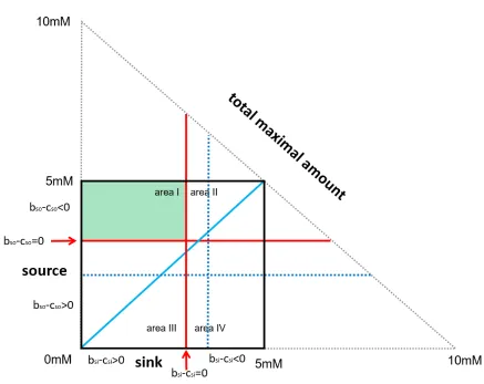
entities forming an ensemble of a source and a sink (figure 1).

Figure 1

Figure 1

My model resembles the Solow model (1) with a saturating production

(utility) function and a linear cost function but with three dimensions and

two parties forming an ensemble capable to transfer substrate internally

under control of the law of mass conservation. The characteristic of the

saturating function does not stand on economic ground but on a similar

biochemical ground which is the Michaelis-Menten kinetic

(V=Vmax*[S]/(Km+[S])) in source and sink. This choice offers a way to

separately (by mutation, 2) vary the steepness (Km) of the initial part and

the height (Vmax) of the flat part of the saturating function. In addition, this

is the basic form of productivity in all organisms. In my recent paper (2) I

examined the evolution of organisms or companies viewed as ensembles

of ensembles with a peaceful and rational behaviour of two Homo

Economicus active only in area I of the transfer space (3) resulting in only

superadditive net profit in symmetric ensembles. Weak asymmetric

ensembles also show peaceful subadditivity in area I (the abstract was a

little short here). Km, Vmax, cost factor (cf) and benefit factor (bf) differ in

source and sink in asymmetric ensembles.

Area I is an area of peaceful transfers though not always superadditive

and reasonable from an ensemble´s viewpoint. However, there is

additional superadditivity in area II and area III (figure 1). This additional

superadditivity comes with two types of additional cost.

1. Force and deception are investments to cross the limit b-c=0 which

inactivates giving and taking behaviour. This time source and sink

are not completely informed and not absolute strong; they can be

overcome. It is therefore possible with a limited investment to force

and deceive them. In a skilful investment the gain for the investor but

not necessarily for the ensemble will overcompensate the initial

investment. Force and deception are an extrinsic cost. This type of

2. An increasing transfer beyond b-c=0 through force and deception

will lead besides additional superadditivity to an increasing amount

of subadditivity reducing the total amount of superadditivity coming

out of area I to III. This will finally lead to complete subadditivity (3,

4). Subadditivity could be characterized as an intrinsic cost. This

intrinsic cost will automatically show up in the later calculations.

These costs above are to be discriminated from the basic cost of the

substrate, i.e. “c”. This type of cost is inevitable connected to the benefit,

“b”. Benefit and cost are inseparable, opposing features of the substrate.

They are two sides of the same coin, in which the cost looks to the past

and presence of the substrate and the benefit looks to the future.

In the absence of a master, force and deception will be used by that party

which has not yet reached c=0. The other party has already reached

b-c=0 and therefore does neither take nor give anymore. The cost of the

investment into force and deception and into countermeasures is not

considered. Source (bso-cso<0) may force sink to take more (figure 2, blue

arrows B, one and two steps from area I into area II but not IV) and sink

(bsi-csi>0) may force source to give more (figure 2 blue arrows A, one and

two steps from area I into area III but not IV). Both, source and sink using

force and deception, will not cross their own limit b-c=0, they will only force

or deceive the other party of the ensemble to do so. Therefore, the

ensemble will not enter area IV.

But here I will investigate a master behaviour. A master is a third party.

The master is not active in catalysis or production. He is either an honest

broker bringing source and sink together in area I (2) or he forces and

deceives both, source and sink, to transfer beyond b-c=0 from area I into

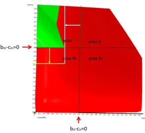
There are two types of masters (4). A conditional and an unconditional

violent and deceptive master. The conditional violent and deceptive

master is at first an honest broker in area I (figure 2 left, green), a

brokerage fee is not considered. He starts violence and deception at the

limit b-c=0 outside of area I to his new limit (figure 2 left, blue area, dotted

blue lines). The unconditional violent and deceptive master will force and

deceive source and sink to transfer beyond b-c=0 already at

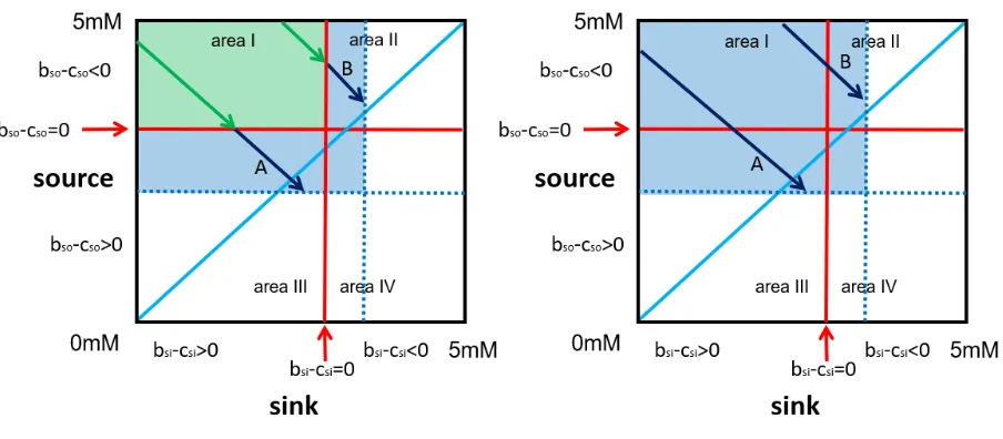
concentrations in area I (figure 2 right, all blue).

Figure 2

Figure 2

A top down view of the transfer space. The dimension net profit of the ensemble points towards the observer. Areas of peaceful transfers (green) and transfers by force and deception (blue) are marked. Exemplary transfers are indicated by arrows (green peaceful, blue with force and deception). All transfers finally end at a blue dotted limit in source and sink, a transfer size of an arbitrary example. Due to mass conservation – the amount taken from source equals the amount given to sink – the arrows run diagonally (volumes and other physical conditions in source and sink are identical). In both cases is the rational limit bso-cso=0 for source or bsi-csi=0 for sink exceeded. Left:

This is an irrational behaviour as in area I force and deception are not

necessary to induce transfers. However, this will produce additional

superadditivity as soon as the border b-c=0 is exceeded. The intrinsic cost

is an even faster growing subadditivity (5).

The effect of introducing a cost for force and deception is not considered

here but was investigated earlier (4, 5). To cross the red lines (bso-cso=0

and bsi-csi=0) will at first increase the amount of superadditivity further.

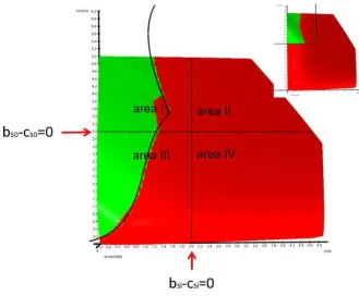
When in symmetric ensembles the transfer will cross the blue line of strict

equivalence (line of mixing of substrate) a small amount of subadditivity

will appear in the centre of the transfer space. This is different in some

asymmetric ensembles (figure 3). A further amount of subadditivity

appears when the red lines to area IV are crossed. This is an area of

complete irrationality where source in benefit domination is forced to give

substrate to sink in cost domination. There are several ways - irrational

and even rational ones - to create subadditivity as described earlier (2, 6).

In the previous paper I observed ensembles with the ability to change the

characteristic values of “b” and “c” (Km, Vmax, bf, and cf) by mutation (or

adjustment, bf as complexity factor, 2). The rational source and sink were

only active in area I (2). In the following examples I observe cases where

the saturating production function “b” and the linear cost function “c” are

fixed again (Km, Vmax, bf, and cf values do not change by mutation).

However, now the limit to which the master will force and deceive source

and sink to transfer to will change. This is understood as a learning

process guided by selection. The master of the ensemble learns to change

the transfer size (size of turnover) beyond b-c=0. Selection will then either

reward the increased transfer size or the increased net profit as result of a

changed (a change can be an increase or decrease) transfer size.

Independent of what selection will prefer, “transfer size” and “superadditive

What is net profit, superadditivity and subadditivity and how are they

related?

According to the Cambridge English dictionary net profit is: “the money

made from selling something after all costs, taxes, etc. have been paid”.

Another definition found (Investopedia): “Profit is a financial benefit that is

realized when the amount of revenue gained from a business activity

exceeds the expenses, costs and taxes needed to sustain the activity”.

In the second definition “benefit” and “cost” are used together like in my

model. Benefit and cost have the same dimension (money or glucose) and

by subtraction we determine the (net) profit. However, in economy a

driving force is to maximize net profit. This stands in contrast to the

behaviour of net profit in my model which behaves identically to the

Solow-growth model. The system develops by redistribution (give cost dominated

substrate, take benefit dominated substrate) towards an equilibrium of

benefit and cost (b-c=0), not a maximal difference. In case the

characteristics of b or c change (e.g. by mutation or invention through

research) the system will occupy in the absence of force and deception a

new stable point; b-c=0. As an alternative I could use the expression

“efficiency” instead of net profit.

I look with a biochemist´s eye on the concept of net profit. Enzyme and

substrate are the core components. The enzyme-substrate complex is a

Janus-headed thing and he is formed in source and sink. Excess substrate

as well as excess enzyme are problematic. Source and sink as separate

compartments will produce product. Substrate may be redistributed

between them to increase productivity in both compartments. The cost is

related to the acquisition and keeping of the substrate and the benefit is

related to the product that will be produced. The size ratio of benefit and

in source and sink and is fixed there but can be changed by relocation.

The point b-c=0 is an optimal substrate to enzyme ratio. Within an

ensemble the substrate is transferred and transformed. It is taken into the

ensemble, redistributed between source and sink to avoid oversaturation

or idleness and then it will be catalytically transformed. Redistribution is

the key step to optimize the net profit within the ensemble. In a symmetric

ensemble with unequal substrate distribution mixing is a simple way to

optimize productivity. An optimal distribution will lead to superadditivity

(additional net profit), a wrong distribution may even worsen the

productivity (subadditivity) in comparison to no redistribution.

Redistribution is a way to change the size of the net profit. Wise

redistribution of substrate is a possibility to maximize net profit.

Superadditivity and subadditivity appear inside the ensemble and are

related to the degree of saturation and kinetic parameters of both sides.

Superadditivity and subadditivity have the dimension “np*mM2_{”, an integral}

of the volume between all possible net profits of an active and an inactive

ensemble in a certain concentration range (here 0-5mM). Net profit is point

like and belongs to a single concentration pair. Superadditivity and

subadditivity also appear here and are the difference of net profit with

transfer and without transfer at a single concentration pair. The dimension

here is np. Although in my definition net profit (np) and super/subadditivity

(np*mM2_{) have different units they are practically identical. The difference}

is the scale; local versus global.

Superadditivity and subadditivity appear in different areas of the transfer

space, sometimes simultaneously. To determine the final balance of many

transfers within the given concentration range superadditivity and

subadditivity are to be subtracted. The final value of an active ensemble

may be superadditive or subadditive in comparison to an inactive

Results and discussion of the results

Superadditivity and subadditivity appear in the transfer space when net

profit of an ensemble without transfer of substrate (inactive) and net profit

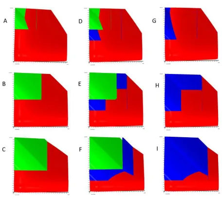
of the same ensemble with transfer (active) are compared (figure 3).

Ensembles can be completely symmetric according to the features of

source and sink (figure 3, row B, E, H) or asymmetric. The transfer in the

active area may be voluntary and induced by force and deception.

The first asymmetric type consists of a weak source and a weak sink, a

weak ensemble (figure 3, row A, D, G). In this ensemble type source does

not like to give (high Vmax or low Km or low cost) and sink does not like

to take (low Vmax or high Km or high cost).

The second asymmetric type consists of a strong source and a strong sink,

a strong ensemble (figure 3, row C, F, I). In this ensemble type source

easily gives (low Vmax or high Km or high cost) and sink easily takes (high

Vmax or low Km or low cost).

The parameters are:

Weak asymmetric ensemble, b-c=0 at 3mM in source, 2mM in sink,

Km=0.5mM, Vmax=5µmol/min in source and sink; cf=(10/7)c/mM in

source and cf=2c/mM in sink, bf=1b*min/µmol in source and sink.

Symmetric ensemble, b-c=0 at 2.5mM in source and 2.5mM in sink,

Km=0.5mM, Vmax=5µmol/min, and cf=(5/3)c/mM in source and sink.

Strong asymmetric ensemble, b-c=0 at 2mM in source, 3mM in sink,

Km=0.5mM, Vmax=5µmol/min in source and sink; cf=(10/7)c/mM in sink

Figure 3

Figure 3

A top down view on several single ensembles and their transfer space. The dimension net profit of the ensembles points always towards the observer, source to the left, sink to the bottom. Red, no transfers, simple additivity; green, peaceful transfers (to the limit b-c=0 in source and sink); blue, transfers by force and deception (1mM beyond b-c=0 as example). Superadditive surfaces are above the red surface, subadditive below (not visible). The end of subadditivity is indicated by a thin green or blue line, an artefact where red, green or blue are of identical value.

Weak asymmetric ensembles: b-c=0 at 2mM in sink and 3mM in source, row A, D, G; strong asymmetric ensembles: b-c=0 at 3mM in sink and 2mM in source, row C, F, I.

Symmetric ensembles: row B, E, H; b-c=0 at 2.5mM in sink and 2.5mM in source.

The ensembles in figure 3 were single ensembles from the type 1 in figure

4. In the following section I will mainly concentrate on ensembles of

ensembles (figure 4-2 and 4-3) like in my previous paper. All necessary

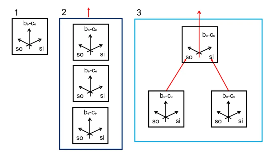
details of the calculations can be found there (2).

Figure 4

Figure 4

1: a single symmetric or asymmetric ensemble. It may be independent or dependent on a conditional or unconditional violent and deceptive master. The net profit of the ensemble is be-ce and in comparing an active and an inactive ensemble we may

observe superadditivity or subadditivity.

2: an unconnected ensemble of ensembles. Three ensembles of type 1 contribute together to the total outcome (red arrow) of either superadditivity and subadditivity or they contribute together to the total amount transferred when the master is interested in transfer fees.

The amount of superadditivity and subadditivity created depends on the

type of asymmetry and the use of force and deception. Superadditivity as

well as subadditivity appear in peaceful ensembles and by conditional or

unconditional violence and deception without or with a master. A mixture

of conditional and unconditional violence and deception is not

investigated. Neither in the single ensemble nor in all three ensembles of

the organism or company as ensemble of ensembles.

Besides a setting where all concentrations are of equal probability there is

also the possibility that a substrate is to both sides of the ensemble either

rare or in complete abundance. The ensemble will then only be active in

area II or area III. We start with the observation of an equal probability for

all concentrations (concentration pairs) in the range from 0 to 5mM in

source and sink of all three ensembles.

Unconnected ensembles:

In the following section every organism is composed of three unconnected

ensembles (figure 4-2). The population contains nine organisms controlled

by nine masters. All nine masters are either conditionally or unconditionally

violent and deceptive. Every organism is made entirely of ensembles of

the type A (figure 3A, all weak asymmetric ensembles) or type B (figure

3B, all symmetric) or type C (figure 3C, all strong asymmetric ensembles)

from the most left column in figure 3. This gives us the basic value of

superadditivity corrected for subadditivity if present. Km, Vmax, benefit

factors (bf) and cost factors (cf) are fixed and identical in source and sink

of all 9*3 ensembles of a population. The masters (conditional or

unconditional) are present but not yet active; this is indistinguishable from

an independent ensemble. Then the masters start to learn to change the

transfer size beyond b-c=0 in source and sink either by conditional or

Transfers of the same size and direction:

The master learns to force and deceive source to give beyond b-c=0

(decrease of substrate concentration) and sink to take beyond b-c=0

(increase of substrate concentration) by the same step size. As result the

superadditive net profit of the ensemble will change. The intersection of

the dotted blue lines in figure 2 moves on a diagonal connecting the

concentrations 0mM sink 5mM source with 5mM sink, 0mM source. The

three starting ensembles in every organism have a maximal range of 3mM

(A), 2.5mM (B) or 2mM (C) to transfer substrate within their respective

borders. Savings, fat reserves, a storage or credit do not exist. Differing

and independent step sizes on source and sink side are later investigated.

Two types of masters are observed: an all conditional violent and

deceptive master (figure 3 D, E, F, figure 5) or an all unconditional violent

and deceptive master (figure 3 G, H, I, figure 6). Every master will be

punished or rewarded by selection for the result of his three ensembles.

The three best masters and their ensembles will have one offspring each,

the three next survive and the last three die. As we observe the evolution

of a population of 9 masters and their ensembles the average of the nine

outcomes (9*3) is depicted according to:

• transfer size (green) changed by mutation, always starts at zero • net profit (blue), a result of the changed transfer, different beginnings

Either the increase of the transfer size or the increase of the net profit is

rewarded in the evolutionary learning process. Observed is side by side

the development of transfer size and superadditive net profit. The outcome

is depicted always with the generation time as x-axis. The y-axis is either

the transfer size (mmol) or the size of the superadditive net profit (np*mM2₎

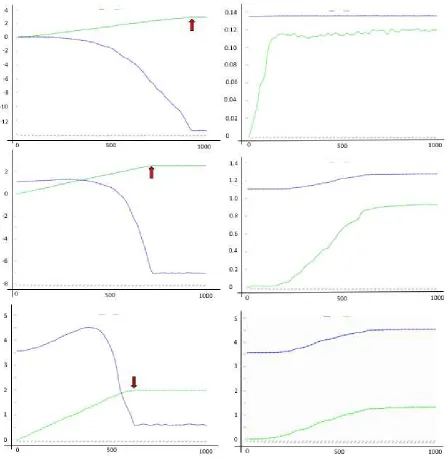
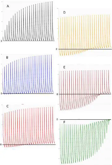
for both evolutionary ratings. In figure 5 we observe the learning process

Figure 5

Figure 5

We look at the average of a population of nine conditional violent and deceptive masters and their unconnected and dependent ensembles of ensembles (9*3) over the time of 1000 generations (x-axis). The colours (blue, green) are not related to the usage of colours in figure 2 and 3. In the left column selection favours transfer size and in the right column selection favours superadditive net profit. The curves show the development of superadditive net profit (blue) and transfer size (green) over (generation) time. The pattern top to bottom is related to the pattern D, E, F in figure 3 (top, weak asymmetric ensemble; middle, symmetric ensemble; bottom, strong asymmetric ensemble). The number on the y-axis is either the amount (mmol) of substrate transferred (green) or the superadditive net profit (blue, np*mM2_{) scaled by}

In the beginning the master is an honest broker. He brings source and sink

together, and they transfer at free will until b-c=0. A brokerage fee is not

considered. Then the master learns that there is more superadditivity or

more substrate to transfer. It is obvious (figure 5) that within 1000

generations the masters learn to increase either transfer size or net profit.

However, the aim to maximize transfer size (figure 5 left column) finds no

limit within the borders of the system independent of the ensemble type

(symmetric, asymmetric). The system comes to an external limit (red

arrow). There, additional substrate is no longer available within the

ensembles and the increase in transfer size stops. The development of

net profit is depressing. Net profit may go through a small or larger phase

of initial increase but in the end net profit will decrease far below the

starting value. This development stops when transfer stops. In two cases

superadditive net profit is negative (subadditive) before the system finds

its external limit. In the strong asymmetric ensemble, the final net profit

stays positive (superadditive) but is far below the starting value (figure 5,

left column, bottom). In the case where selection favours a better net profit

(figure 5, right column) the system finds an internal limit and equilibrium.

Net profit is maximized and then the increase of transfer size stops

because more transfer would decrease the net profit again which is

punished. In the weak asymmetric ensemble, the increase in net profit is

barely visible (figure 5, right column, top) as the amount of subadditivity

produced by this type of asymmetry is already considerable at the start.

The starting value of superadditive net profit is 1.35 np*mM2 _{and does not}

increase detectable while transfer size increases only a little. The situation

in figure 3 D (transfer size of 1mmol) is a possibility only for the case where

selection favours transfer size. The net profit of the whole ensemble is

already negative at that transfer size.

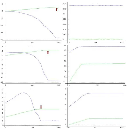
Figure 6

Figure 6

The observations with the unconditional violent and deceptive masters

(figure 6) are very similar to the conditional violent and deceptive masters.

But there are a few interesting differences. It is already known from my

older work (5) that the superadditivity of this master will increase faster

and to a higher level but will then also decrease faster and steeper. This

was observed with symmetric ensembles.

Remarkable is the observation that within the weak asymmetric ensemble

(figure 6 right column, top) there is no increase in transfer size and

superadditive net profit. It was already clear from figure 3 that the amount

of subadditivity produced is larger within an ensemble of an unconditional

violent and deceptive master in comparison to a conditional violent and

deceptive master. The amount of subadditivity is of the same size as the

amount of superadditivity. The system can no longer react as every

movement of the limit in either direction away from b-c=0 (shrink or grow)

will increase superadditivity and subadditivity or decease superadditivity

and subadditivity to the same extent.

The observations in figure 5 and figure 6 also explain a common

misunderstanding of ideologists. In the beginning of some ensemble types

an increase of transfer size will increase net profit. Simple minds start now

to think in straight lines. However, there is an early end to this lockstep

and that is not even the external limit. The simple thinking must end when

net profit starts to break down. That is the point where realists and idealists

separate.

In the preceding paper (2) it has already been learned that recombination

does not change the basic outcome of the results. Evolution with

recombination is just faster and this is well known from Biology. The data

Transfers of different size and direction:

In figure 5 and 6 the growth of transfer size and net profit of a weak

asymmetric ensemble is neglectable or not present at all (figure 5 and 6,

right column, top picture). The reason is the considerable amount of

subadditivity produced right from the very beginning in combination with a

master linking the step size and direction on the source side to the step

size and direction on the sink side. This is changed now. On the source

and sink side different step sizes and different directions on either side of

b-c=0 are possible. Every single transfer is still controlled by the law of

mass conservation. An illustration of this idea is presented in figure 7.

Figure 7

Figure 7

The transfer space is a model that could be called an “outer model” or an

objective, factual model. Such facts are Km, Vmax, bf, cf, the substrate

and it´s concentration range. The outer model is inhabited by up to three

parties. The outer model is the reality for source, sink, and master. The

three parties must decide whether they become active or stay inactive. For

this they need their own model. I call this an “inner model” or a subjective

model. The inner model used by the master could be the only model to

match the complexity of the outer model as the master is no component

of the transfer space.

To determine concentrations is a simple way to orient within the transfer

space. The inner model of a Homo Economicus regarding a concentration

as a limit to give (source) or to take (sink) can come to the same result as

the outer model; b-c=0 i.e. 2.5mM in a symmetric ensemble. Therefore,

Homo Economicus acts reasonable and rational. But that is also the

starting point for conflicts. Source and/or sink must be forced or deceived

to change their reasonable behaviour. Source and sink could have other

inner models than the model of a Homo Economicus. Conflicts would be

absent if source and sink would have no inner model at all. The possibility

of superadditivity and subadditivity would still exist as this depends on the

outer model. Whether the source and sink are active or not would then

depend on the on the inner model of the master. Whatever inner model

source and sink would use to guide their behaviour, conflicts will only arise

when the inner model of master and source and sink differ. Inner models

can be the cause of subadditivity in source and sink even in the absence

of a master because the inner models can misguide source and sink within

the outer model, their reality.

In the preceding section I observed two intentions with different

complexity: more transfer (increase concentration limit in sink, decrease

decrease concentration limit only when net profit will increase). The

determination of a net profit is a very challenging task in comparison to the

determination of a concentration or a concentration difference. The

simplicity or complexity comes from dimensionality of the model, the

necessity to obtain the appropriate information (an additional cost) and to

behave accordingly.

The transfer space is a three-dimensional model. The inner model of

source and sink may range from a single concentration (a point, dimension

zero) to a two-dimensional model with the assumption of certain values (b

or c). Source and sink are two-dimensional entities. Although source and

sink may use such complex models (b-c=0 as limit) they are not

necessarily superior to a simple limit like a concentration. In case the cost

function or the benefit function come from wrong assumptions the limit will

be wrong, too. The model of the master may range from a single

target-concentration in source and sink to a three-dimensional model or of even

higher dimensionality than the transfer space. A model with higher

dimensionality than the transfer space will not help but confuse as it will

result in overfitting.

In a past paper (4) I already introduced a master with a complex behaviour

and intention. His aim was to maximize superadditivity by avoiding

subadditivity. I called him “prudent master”, a designation and behaviour

introduced by Adam Smith. In symmetric ensembles the prudent master

will not cross the line of strict equivalence or mixing. He has a linear inner

model. This is a very adaptive, demanding, and intelligent strategy as he

can´t stick to a fixed value of a substrate concentration like a wise limit (4)

which is a constant inner model. In figure 8 we observe again a type of a

prudent master but now with a nonlinear inner model suitable for an

Figure 8

Figure 8

A single weak asymmetric ensemble is shown top down (source to the left, b-c=0 at 3mM; sink at the bottom, b-c=0 at 2mM; net profit of the ensemble towards the observer). After 2000 generations the master has leaned to optimize superadditive net profit with two sinus functions as limits (black lines) of his inner model. Although source and sink have no inner model, the limit b-c=0 is marked in source and sink as this is still a fact in the outer model. Force and deception are therefore not necessary. The small inset is the starting condition at generation time zero. The master will induce giving and taking left of the black line, producing only a small amount of subadditivity in area I and a large amount of superadditivity in area III.

In figure 5 and 6 the superadditive net profit of the ensemble of ensembles

with asymmetric weak ensembles was about 1.35np*mM2 _{on average of}

the whole population and could no longer improve. The system was

frozen. The superadditive result of a more complex limit discovered by an

evolutionary learning process is 7.9np*mM2 _{within a single ensemble}

(figure 8). The starting generation began at the former borders b-c=0

and in sink separately. The letters a, b, c, and d are parameters which are

changed during the evolutionary learning process. They are mutated with

a random, normal distributed value and an expected value of zero and a

standard deviation of 0.01. S is the amount of substrate in source and sink

of the concentration pair at the limit. The concentration pairs along the

diagonal (to the upper left of this pair) will result in a certain amount of

superadditivity or subadditivity if the values before and after a transfer are

compared. In contrast to the starting conditions (figure 8, inset)

subadditivity within the borders is reduced and superadditivity is

increased. With a more complex limit (a*sin(b*S+c)+d + e*sin(f*S+g)+h)

7.9np*mM2 _{could not be improved further.}

In figure 8 it is demonstrated that within an ensemble of a source and a

sink without an inner model the master can freely set limits without using

force and deception. The complex limits he uses, simultaneously reduces

subadditivity and increases superadditivity considerably in comparison to

the starting conditions. This time the prudent master will not allow source

to give to sink beyond certain values as this will produce subadditivity. The

master will reduce the amount already given by source to sink in the

starting configuration. The master´s inner model is again shaped by an

evolutionary learning process and selection. Every increase or decrease

in transfer size will result in an increase or decrease of superadditive net

profit. Selection will only reward inner models resulting in an increase of

the final balance (superadditivity minus subadditivity). This can be

achieved by reduction of subadditivity and by increase of superadditivity.

But imagine you are a two-dimensional entity (source, sink) with your own

inner model. You observe how your limits are ignored, violated and

unreliably changed when concentrations change and this appears biased

towards another party; conflicts will be the result. Source will not accept

to the limit bso-cso=0. Furthermore, also sink will be angry because sink

could use this substrate to get closer to its own limit bsi-csi=0. This is valid

for area I and II. On the other side (area I and area III) the master will

increase the amount of substrate taken from source and given to sink. On

this side there is still plenty of additional superadditivity. However, this

would be against the interest of the source as the source on this side is

forced to give beyond the limit bso-cso=0. For many different reasons a

rational inner model makes source and sink oppose the prudent master.

Prudence would have to be enforced by force and deception (conditional

or unconditional) as “prudence” relates to the aim and not to the measures.

The prudent master tries to maximize superadditive net profit. Therefore,

the prudent master is even able and willing to decrease the transfer size.

The master who lives on transfer fees is unable to understand this and

unwilling to do so.

The model implies another possible idea of the master. He is capable to

decrease area I on one side (area I to area II). That is very helpful in an

asymmetric ensemble like figure 3 A, D, G. Here, the decrease in transfer

size on one side and the increase in transfer size on the other side will

synergistically affect the overall increase in superadditivity (figure 7 and

8). What happens if the master will decrease the size of area I on both

sides? In a symmetric ensemble such a behaviour of the master would

have a different effect and purpose. Area I with only superadditivity would

become smaller; a harm to the ensemble not reaching the full potential of

superadditivity. Source and sink must look for another sink or another

source to reach b-c=0. This could be the true motivation of the master. The

master may be biased towards a new source or sink. He will endure the

loss either as a smaller transfer fee or a smaller net profit to share. Later

he will then enjoy the better access to net profit share or transfer fees with

Connected ensembles - substrate probability:

Until now the different concentrations of substrate in source and sink had

the same probability. At a given concentration pair in source and sink a

definite net profit and a fixed superadditivity or subadditivity is produced

when the net profit before and after a transfer is compared. These point

like portions of superadditivity or subadditivity are of different size over the

concentration range. Some size classes appear more often than other size

classes. A size and frequency distribution of this local portions of super-

and subadditivity can be observed; a spectrum. This has not been

important before as the ensemble was single or unconnected and only the

total amount of superadditivity minus subadditivity was calculated. As soon

as connected ensembles (figure 4-3) are observed this is different. Now

the top ensemble will receive a spectrum of superadditivity and

subadditivity. Only the basic ensembles have an equal substrate

distribution over the whole concentration range. This is the only place

where substrate enters from the outside with equal probability. Then the

substrate is handed over within the ensemble. The decrease in substrate

concentration handed to the top ensemble is compensated by a single

benefit factor, here bf=6 (2). Now bf has features of a complexity factor.

The result is a higher substrate concentration range (again 5mM) for

source or sink but now as a spectrum and no longer a uniform distribution

with equal probability for all concentration pairs. The production of

superadditivity in the top ensemble depends on a high input on the source

side and a low input on the sink side. The reverse input may result in

subadditivity in the top. This is different when transfer size is the aim. Then

the transfer will become large on both sides of the top ensemble. However,

the result in the top ensemble depends on what will increase first and in

what sequence and size. The observable spectrum in a single symmetric

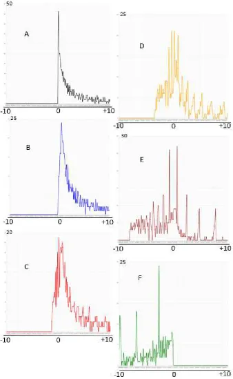
The spectrum in figure 9 is a two-dimensional representation of a

three-dimensional distribution – a repeating cross section. The active part of the

transfer space is divided by a 25*25 grid into 625 single columns. The

numbering starts at 5mM source, 0mM sink and ends at the actual transfer

limit, e.g. 2.5mM source, 2.5mM sink in figure 9A or at 0mM source and

5mM sink in figure 9F. The size of superadditivity and subadditivity is

displayed on the vertical axis, the position number between 1 to 625 on

the horizontal axis. Figure 9A is the starting condition, the ensemble has

transferred at free will or with a master in one step to the limit b-c=0 (only

superadditivity, 0mM to 2.5mM in source and sink). In 9B to 9F we observe

how subadditivity develops and the spectrum of superadditivity changes

while the master increases transfers in steps of 0.5mM beyond 2.5mM to

finally 5mM. It is easily visible how subadditivity develops below zero. In

9F the ensemble is completely subadditive.

The spectrum of superadditivity and subadditivity handed over to the top

ensemble is dependent on the mutational step size (normal distributed)

and the location and sequence of the mutational steps (source side or sink

side within the same ensemble, in case they are independent like only in

figure 8). Therefore, the sequence of differently sized mutational step sizes

in source or sink will lead to a unique historical process of the evolution of

a connected ensemble. Every specific mutation in step size will result in a

different spectrum and in return in a different development of super and

subadditivity in the top ensemble. As the Michaelis-Menten equation is not

defined in the negative substrate range the subadditivity is set to zero in

the connected ensemble in figure 11. In economics this might be different

as the subadditivity of a lower level could be felt as a negative income of

a higher level. Under real conditions only single concentration pairs will

occur per timepoint within one ensemble of ensembles and the result will

Figure 9

Figure 9

Figure 10

Figure 10

Connected ensembles – evolutionary behaviour:

Every organism (company) in the following part is composed of three

connected ensembles (figure 4-3). The top ensemble will receive a

spectrum of substrate concentration from the two lower levels (figure 10).

Only the two basic ensembles have equal substrate probabilities in the

range of 0mM to 5mM substrate. The benefit factor for the top ensemble

(a complexity factor of 6 like in publication 2) compensates for decrease

in concentration from the lower level to the top level because Km, Vmax

and cf are the same in the basic and top ensemble. Superadditivity can be

interpreted here as both, efficiency or additional net profit. The substrate

entering the ensembles at the bottom is distributed in a way that there will

be better efficiency or additional net profit. Either substrate is left over after

superadditive redistribution and is then used in a higher level or additional

net profit after redistribution of substrate can be invested in a higher level.

The higher level is also understood as a higher level of complexity. This is

comparable with the investment of money (glucose) either in workforce

(muscles) or computer-controlled automatization (brain). The leverage of

the same substrate in the higher level is larger than in the lower level. It

should not be forgotten that within the unconnected ensembles three times

two substrate portions are consumed while in the connected ensembles

only two times two substrate portions are consumed.

A master living on transfer fees (figure 11A, the y axis is transfer in mM)

will depend on the transfer size in the ensembles at the bottom where he

will enforce transfers by force and deception and will be rewarded for an

increase there. The master here is unconditionally violent and deceptive.

Besides the increase in transfer in the ensembles at the bottom we are

going to observe the production of net profit of the top ensemble. A transfer

there by force or deception is absent. A population average of 9 connected

observed. According to the transfer size the best three have one offspring

each, the next three survive and the last three die. The average (net profit

and transfer size) of the population is observed.

A master living on net profit (figure 11B, the y-axis is superadditive net

profit – mM2_{*np) will participate in the net profit of the top ensemble where}

no force or deception is used and will be rewarded and observed

accordingly. He will use force and deception in the ensembles at the

bottom to induce transfers but controlled by net profit in the top. A

population average of superadditivity within the top ensemble of 9

connected ensembles (9*3) with 9 unconditional violent and deceptive

masters is observed. According to net profit production the best three have

one offspring each, the next three survive and the last three die. In parallel

the average transfer size within the bottom level ensembles will be

observed.

In connected ensembles the two different strategies of masters (10A - live

on transfer fees, 11B - live on net profit) reveal very different results. In

general, the development of a connected ensemble over the generation

time is no longer very reproducible. Every run is unique but reveals a

typical behaviour.

In figure 11A the connected ensemble starts superadditive, develops

increasing subadditivity which will later reverse but will stay subadditive at

the end of transfer. When the transfer arrives at the maximal amount, the

system shows only small fluctuations. Locking at three times three

connected ensembles (figure 11A, inset), a transitory change (alternating

increase and decrease) in superadditivity/subadditivity is observable as

long as transfer will go on. At the end of this phase the system is

Figure 11

Figure 11

In figure 11B transfer does not go far beyond 1mM. The reason is that the

master is controlled by net profit. Because of the nature of the spectrum,

there is an ongoing improvement of net profit although an increase of

transfer in the lower levels is barely detectable. Superadditive peaks on

the source side of the top ensemble coming from the basic ensemble are

combined with subadditive (set to zero by definition) areas on the sink

side. Evolution moves upwards with waiting times (plateaus) from smaller

peaks to larger peaks in the vicinity. This leads to a step wise and ongoing

increase in superadditivity. This is achieved by minimal changes of the

spectrum via minuscule changes in the transfer size on source and sink

side. Net profit as bench mark leads again to an internal equilibrium of

transfer. This equilibrium is still able to improve!

Other reasons for different substrate probability:

In the past I have always used equal probability for all concentrations

(concentration pairs) entering the ensemble from the outside; here in the

range from 0 to 5mM in source and sink. This might be viewed as an

artificial situation as in nature the concentration of substrate will be

probably either high for source and sink or low for source and sink.

Substrate will be cost dominated for both sides as there is plenty of

substrate or substrate will be benefit dominated for both sides as substrate

is scarce.

In figure 12 I look at an illustration of this idea. A single symmetric

ensemble has either a substrate concentration higher than 2.5mM for

source and sink (area II) or lower than 2.5mM for source and sink (area

III). The symmetric ensemble exists either in area II or in area III (for

Figure 12

Figure 12

In previous examinations I always compared masters in control of the

whole transfer space. This is different here. Due to the non-uniform

substrate distribution the master only controls a part of the transfer space.

He is either in control of a saturated ensemble in area II or a hungry

ensemble in area III. If I want to compare such masters, I must take care

for equal starting conditions. Why are the starting conditions unequal? At

a concentration of 5mM in source and 0mM in sink the transfer space

contains a certain amount of substrate. At 5mM in source and 5mM in sink

the ensemble contains the double amount of substrate in identical volumes

for source and sink. Equal conditions are present when always the same

amount of substrate is present within the whole ensemble. This is the case

in my example at a concentration of 10mM in source plus sink (figure 12).

Now I can compare the two masters.

The concentration range is now triangular shaped. Even in a symmetric

ensemble the four areas are no longer of identical size and shape.

However, there is now a just access to the same maximal amount in

source and sink.

In case source and sink have no inner model, the master will steer them

without problems. In case source and sink are two Homo Economicus the

master must force them to give (source, area III) or to take (sink, area II).

Force and deception start at b-c=0 (border between area I and II or border

between area I and III). The cost of force and counter force is omitted. Now

I am going to compare two masters who rule either an ensemble with

abundance (area II) or deficiency (area III). The masters are no prudent

masters. Starting at b-c=0 they learn that more substrate can be

transferred, and more net profit can be made by force and deception. We

observe the balance of super- and subadditivity. It is here no longer

possible to differentiate the unconditional violent and deceptive master

Figure 13

Figure 13

Figure 14

Figure 14

Figure 15

Figure 15

In figure 13 to 15 we compare two masters using force and deception.

They live under two different conditions i.e. lack in area III and surplus in

area II. In addition, we lock at three different types of ensembles, two

asymmetric ensembles and one symmetric ensemble. The transfer size is

limited to maximal 2.5mmol in steps of 0.05mmol beyond b-c=0. The limit

b-c=0 differs within the three figures (figure 13, 14, 15)!

In a weak asymmetric ensemble (figure 13) the master who is in control of

the ensemble which has to deal with a lack of substrate is always doing

better. This is only true for the observable part of the subadditive range. In

the symmetric ensemble (figure 14) the master in control of the ensemble

with lack of substrate is in the beginning doing better. Later, when

subadditivity starts to develop in both ensembles, the master with an

ensemble active with surplus of substrate is doing better as subadditivity

does not develop so dramatic. Interestingly there is a transfer size

(1.65mmol) where the ensemble with surplus of substrate is still

superadditive while the ensemble with lack of substrate is already

subadditive. Finally, in an asymmetric ensemble with a strong sink (figure

15) it is interesting to observe that in the beginning the ensemble with

surplus is doing still slightly worse than the ensemble with lack of

substrate. However, later in the observed transfer range (2.5mmol) the

master with the ensemble in surplus will dominate with superadditivity

while the master and his ensemble with lack of substrate will be completely

General Discussion

The roots of the idea

The idea of a complete balance within the transfer space of a source and

a sink goes back to Antoine-Laurent de Lavoisier (born 26.08.1743 –

executed 08.05.1794), economist and chemist. He is acknowledged as

one of the fathers of modern chemistry. He changed chemistry from a

qualitative to a quantitative science by introducing the mass balance. As

administrator of the “Ferme Générale”, a tax farming company in the

pre-revolutionary France, he was used to the concept of a balance sheet. In

his experiments e.g. with mercury(II) oxide (HgO) he understood that he

not only had to observe the weight of the vessel where mercury(II) oxide

would decompose to mercury upon heating but he also had to control the

weight of “the other vessel” - the surroundings - to make a complete

balance. He collected the developing gas (oxygen) and found that the

mass of the starting material (mercury(II) oxide) was identical to the sum

of the mass of the products (mercury and oxygen).

The same is simply repeated here again. We do not only have to observe

what happens in one enzyme-filled vessel (cell, organism, company or

country) when we put substrate in; we also must observe the vessel where

this amount of substrate came from. For simplicity this vessel should be

as identical as possible. A complete balance should include both vessels

connected with each other as source and sink. The mass (and energy) is

conserved during the transfer. The productivity after a transfer from source

to sink with its non-linear, saturating behaviour will show us new features

(superadditivity and subadditivity) in comparison to the condition “no

transfer”.

This may appear to some readers like the parable of the broken window

But my model is not about a microeconomic opportunity cost. It is not about

“here or there” in one party. The paper is about “before a transfer and after

a transfer” within an ensemble of the same two parties; a source and a

sink.

Quantity and Quality

A function in mathematics is the model of how a quantity depends on the

variation of another quantity; y=f(x). In the physical world we often face the

fact that a quantity depends not only on a single other quantity but usually

on many others with different functions; y=f1(x1)+f2(x2)+…+fn(xn). Solid

experiments try to control complex dependencies either with the skilful

exclusion of such effects or by control experiments.

A second possibility is that a single quantity (x1) may have different

features (functions); y=f1(x1)+f2(x1)+…+fn(x1). Here it is not possible to

reduce the experiment to one single dependency. We may observe in

controls a first function with a positive influence and a second function with

a negative influence on the outcome; y. Therefore, we sometimes observe

an unexpected change (“Nach fest kommt ab.” - Don´t push too hard.)

while we change the quantity e.g. a linear force increase.

Experience is teaching that “more is not better” or that there is the

possibility of “too much of a good thing”. This is often discussed as a

problem of quantity versus quality. But what if quality is a combination of

two independent features connected and related by a common quantity?

Quality emerges from the relative share of the two different features. In

case the quantitative nature of a first feature is obvious and easily

determined and the quantity of the second feature is difficult to determine,

entanglement (7) the kin and its fate for the balance of all identical genes

appears as a quality in comparison to the self as a quantity and as an

orthogonal dimension. The “two times two” features (b, c) in entanglement

(ef, degree of informational identity) are connected by a single substrate

and the two pairs of benefit and cost are orthogonal as are source and

sink, i.e. parent and offspring. The effect of the success factor (sf, an

external factor indicating the probability of survival) in entangled,

symmetric parties is asymmetry. In reverse, the success factor can

compensate for asymmetries in Km, Vmax, cost factor and benefit factor.

How can we judge where we are in “quality” (good – too much good) when

we measure only a single feature of the quantity (thing)? – Not at all! We

must determine both aspects (features) of that quantity.

“Too much of a good thing” implies the presence of an optimum or at least

a change of character. “Much” will be good - better than little - but “too

much” will be no longer as good. There are many functions producing

optima or go from positive values to negative values. I create such

behaviours with two monotonously rising functions both dependent on the

quantity x1.

Let there be two features of the quantity - e.g. a substrate. The two

features of the substrate (x1) are a benefit with the function (f1) and a cost

with the function (f2); f1(x1) and f2(x1). When we increase the amount of the

substrate the two features independently and monotonously rise and

follow their respective functions. In case they intersect we will see on one

side of the intersection values of function f1 dominate over values of f2 and

on the other side we will see values of function f2 dominate over values of

f1 (change of character). When we look at each single function (feature)

we will always see an improvement. But the improvements stand in

physical dimension we can subtract the values (y=f1(x1)-f2(x1)), in case

they are measured in different physical dimensions we divide them (y=

f1(x1)/f2(x1)). The intersection in subtraction will be zero and in division one.

Depending on the sequence (f1,f2 or f2,f1) and the shape of the functions

we may observe a maximum or a minimum somewhere.

Why is net-profit such an important concept?

In the investigated evolutionary learning process two types of evolutionary

ratings are examined. On one side I use a positive relation between

success and amount; “more transfer is better”. In the alternative rating I

use a positive relation between success and superadditive net profit;

“more superadditive net profit is better” which is basically more net profit

in a wide range of concentrations. It is generally acknowledged that net

profit is the most important and most used criterion to judge whether a

company is successful or not. The same could be said about organisms

when we compare e.g. the consumption of energy (glucose consumption

as cost c) of a hunting predator and the gain of energy equivalents (protein

and fat of the prey as benefit b).

Why is net profit such an important measure? I think it would be too simple

to argue from a quasi-evolutionary standpoint like: “Other criteria to judge

the success in economics and in biology have not proven to be as effective

as the use of the concept net profit”. This is not an explanation, this is only

an observation. Why do we make this observation?

From my results it seems that we reach independently of what we observe

(amount transferred or superadditive net profit) only with superadditive net

profit as selection criterion stability. Turnover as criterion will always go to

negative (net profit) values. With net profit as criterion the ensemble will

find an internal point of stability. The external limits of the ensemble are

not exceeded. Transfer size as criterion will always exhaust the capacity

of the ensemble and blow up the limits. Wise limits may be violated by

both criteria.

In connected ensembles there are additional observations. The increase

in net profit takes place in steps. Source and sink at the bottom should go

different directions. The ensemble on the source side should deliver much

superadditivity, the ensemble on the sink side should deliver only a little

superadditivity or deliver subadditivity. Most amazing is the effect of the

spectrum of the super- and subadditivity in masters living on transfer fees.

While there is increasing transfer there will be “something to observe”. If

such a master is going to observe the net profit - which is basically not his

personal interest - he will be very surprised. An increase in transfer may

increase superadditivity and in the next step of increase it will produce

subadditivity.

“Certain forms of knowledge and control require a narrowing of vision” (8).

This narrowing of vision is the starting point for a master to fail. What

appears useful under a certain condition may be complete nonsense in

the direct adjacent condition. Linear minds only succeed to extract simple

patterns from complex, nonlinear patterns. Those simple patterns produce

easy to understand, convincing models but they fail the test of reality –

repeatedly. The reason for the repetition of mistakes is the lack of insight

into cause and effect and the lack of a sense of personal responsibility and

Culture, Religion and political Ideology

A Greek proverb says: “A society grows great when old men plant trees

whose shade they know they shall never sit in.” Culture seems to be an

integrated system of force and especially deception in man to create

superadditivity outside of area I. However, this will include irrational,

self-harming economic behaviour on the level of the single party.

Two advances are immediately obvious:

• additional superadditivity of the ensemble when the limits are carefully chosen and the additional costs are controlled;

• the ensemble can be active when substrate is benefit dominated for source and sink (area III) or cost dominated for source and sink (area

II) simultaneously (figure 12 – figure 15). An ensemble of rational

entities (two Homo Economicus, strong and informed) would be

inactive under such conditions.

It seems to be a very probable situation that the substrate distribution is

for source and sink similar; either both lack substrate dominated by benefit

(b-c>0) or both have a surplus of substrate dominated by cost (b-c<0).

Religion and ideology are deceptive concepts to induce transfers beyond

the rational limit b-c=0, outside of area I. The specific deception will

convince someone to take a cost dominated substrate or to give a benefit

dominated substrate without expensive and harming force. This will only

work if benefit and cost - the inseparable connected features of the

substrate - are separated within the ideological framework. Even in

science there are attempts to construct a world where benefit and cost are

separated (9, 10) and net profit is no benchmark. The basic assumption in

all this scientific teaching is the existence of a phlogiston-like concept

in biology is based on an ideologically and religiously founded emotional

rejection of the rational and self-limiting net profit. Phlogiston-like

constructs and miracles always vanish when a complete balance is

implemented.

The ability of an ensemble to find a rational and sustainable internal limit

using net profit as benchmark is a danger to an external instance (master)

living not on increased net profit of the ensemble but on transfer fees.

Therefore, this type of master hates the idea of net profit. His teaching, the

whole culture he will create, will praise emotions and irrational behaviours

of role models and deter and discredit rational behaviour. He will either

avoid scientific proof and claim higher values and believes to discourage

and break resistance or scientific proof is claimed although the scientific

method is not followed as the predicted progress reveals as an endless

failure. This type of master is interested to increase the size and amount

of transfers. The ensemble, dependent on its internal superadditivity, is

doomed as the unlimited and irrational transfer will increase subadditivity

until all superadditivity is consumed. The master with his ideology moves

on as archenemy of the free man (Homo Economicus) and ensembles

formed by him. Homo Economicus – as an ideal strong and informed – will

never fall prey to force and deception thus avoiding area II, area III, and

especially area IV of the transfer space. His freedom of decision to stay

away from areas II, III, and IV comes at a price. Such ensembles can´t be

active outside of area I. This inactivity is a strategic weakness and comes

from strength and knowledge; what an irony, what a tragedy.

But maybe that is the difference between humans and animals. The inner

model of animals shaped by evolution may be very identical to reality (the

outer model). Therefore, animals behave like a Homo Economicus. This

realistic inner model, this genetic a priori knowledge, is at least partially

models and therefore can be active outside of area I. Outside of area I

superadditivity is produced by harm to at least one party. This is rewarding

to the master and maybe to the ensemble they are a part of as long as

superadditivity dominates. To compensate the harm reciprocity or a

constant natural overproduction is necessary. Replacement of burned

parties by a new generation will stabilize the ensemble and prevent a Nash

equilibrium. It should not be forgotten that the balance we observe is made

within a steady state equilibrium of a biological system constantly powered

by the sun; this is not a closed system. Although we observe in Biology

and Economy an open system mass and energy will be conserved in its

very basic meaning – nothing comes from nothing and nothing vanishes

into nothing. A complete balance will always show this.

Literature

1. Solow RM (1956) A Contribution to the Theory of Economic Growth. The Quarterly Journal of Economics, Vol. 70(1) 65-94

2. Friedrich T (2018) Evolution towards higher net profit in a

population of ensembles of ensembles leads to division of labour. MPRA_paper_85517

3. Friedrich T and Köpper W (2013) Schumpeter´s Gale - Mixing and compartmentalization in Economics and Biology.

MPRA_paper_45405

4. Friedrich T (2015) The limits of wise exploitation in dependent and independent symmetric ensembles. MPRA_paper_68250

5. Friedrich T (2016) Aquila non captat muscas: Homo Economicus between exploration and exploitation. MPRA_paper_75601 6. Friedrich T (2014) Work cycles of independent ensembles.

MPRA_paper_55090

7. Friedrich T (2014) Entanglement by Genes or Shares - Hamilton´s rule of kin selection revisited. MPRA_paper_60267

8. Scott JC (1998) Seeing like a state. How certain schemes to improve the human condition have failed. The Yale ISPS series 9. Nowak MA (2006) Five rules for the evolution of cooperation.

Science 314:1560-1563