Maximum Load Balancing with Optimized Link Metrics
Touraj Shabanian, Massoud Reza Hashemi, Ahmad Askarian
Department of Electrical and Computer Engineering, Isfahan University of Technology, Isfahan, Iran. Email: [email protected], [email protected], [email protected]
Received 2012
ABSTRACT
Traffic engineering helps to use network resources more efficiently. Network operators use TE to obtain different ob-jectives such as load balancing, congestion avoidance and average delay reduction. Plane IP routing protocols such as OSPF, a popular intradomain routing protocol, are believed to be insufficient for TE. OSPF is based on the shortest path algorithm in which link weights are usually static value without considering network load. They can be set using the inverse proportional bandwidth capacity or certain value. However, Optimization theory helps network researchers and operators to analyze the network behavior more precisely. It is not a practical approach can be implemented in tradi-tional protocol .This paper proposes that to address the feasibility requirements, a weight set can be extracted from op-timization problem use as a link metric in OSPF. We show the routes that selected in OSPF with these metric distribute the traffic more close to optimal situation than routes from OSPF with default metric.
Keywords: Component; Formatting; Style; Styling; Insert
1. Introduction
This In recent years, the use of the Internet as communi-cation infrastructure for different telecommunicommuni-cation applications has been growing significantly. Because band-width is one of the most important requirements of these applications, network hardware should support band-width management techniques. Traffic engineering (TE) is a bandwidth management technique that considers different objectives such as maximum throughput, mini-mum congestion and load balancing in the network. TE puts the traffic where network bandwidth is available [1]. TE with the objective of load balancing can reduce maximum link utilization (MLU) and increase bandwidth efficiency (BWE). Because considerable delay may oc-cur at congested links, reduction of end to end delay can be achieved as a side result of load balancing.
Destination-based routing is not flexible for TE, and so it is highly susceptible to congestion. Because of this reason the concept of TE was developed mostly in MPLS-based networks [2,3]. MPLS-based TE can op-timize traffic distribution using dedicated label switch paths (LSP). The capability of explicit routing and arbi-trary traffic splitting are the most important features of MPLS TE. But the MPLS has not been widely deploy Rapid increase in network traffic especially that of new applications which require QoS guarantees, has encour-aged the network providers to apply IP based TE with different objectives. The main idea of IP-based TE is to find a set of weights that optimizes a specific objective
function. If the objective function is the total link cost, the constraint of equal cost multipath (ECMP) causes the problem to be NP hard [4]. Different near-optimal heu-ristic algorithms based on local search were proposed to solve this problem [4].
One approach for analyzing the TE problem is formu-lating it with optimization theory problems. If we con-sider load-balancing as an objective of the optimization problem and consider the amount of traffic load on all links that belong to a specific session as the problem outcome, the solution of such problem is the path of each session that results in minimum congestion.
im-proves bandwidth efficiency and reduces network con-gestion and also leads to a substantial reduction in the end to end delay.
2. Problem Statement
First, Different TE objectives lead to different objective functions of optimization problem. We consider load balancing as an objective of traffic engineering so the objective function of the optimization problem is to mi-nimize MLU (maximum link utilization). Consider the linear optimization problem that is called first primal problem (PRIMAL_I) with the following notation. A connected graph is given. is a set of edge capacities and is a set of source- destination pairs for each session . Is the total amount of session traffic. The amount of traffic in link that belongs to session is . So the problem is: , , :( , ) :( , ) , , , min (1) (2) 0 . . (3) 0 (4) i k k
i j j i i j i j A j j i A
k i j i j k K
i j
MLU
D i sourse
X X D i destination
o w
X C MLU
X ∈ ∈ ∈ = − = − = ≤ ≥
∑
∑
∑
Constraints (2) are flow conservation constraints that are derived from network topology. Constraint (3) ensure that link flows do not violate link capacity and (4) says that link flows are nonnegative. The PRIMAL_I solution specifies the , and so we have the optimal path with arbitrary splitting for all sessions that minimize MLU. Our objective is to find a practical method suited for IP networks that forces the traffic to go through a set of op-timal paths. To achieve this goal we should find a set of new link metrics such that all paths which are specified by PRIMALI problem can also be obtained by the short-est path algorithm in regard to the new metrics. It means that if Xijk>0, then link should be selected by
ses-sion k according to the shortest path algorithm. Here we assume that the shortest path algorithm is OSPF that supports Equal-Cost Multi-Path (ECMP).
The load balancing methods introduced in [6,7] are based on primal optimization problem. In this paper we consider the dual optimization problem (DUAL_II) which is obtained with respect to Lagrange Multipliers. In other word we aim to distribute traffic by determining the links weight. And It will be shown that the Lagrange Multipliers comparable with constraint (3) can be inter-preted as OSPF link metrics that satisfy the load balanc-ing objective. Link metric in OSPF protocol must be an integer between 1 and 65535 but we will show in section IV that the Lagrange Multipliers that are obtains from the
solution of DUAL_II problem and comparable with con-straint (3), do not satisfy this range in general. So the following definition gives us the choice of an alternative weight set.
Definition 1: Two weights set { }L1 i i
W= w = and
{ }L1 i i
W′= w′ = are equivalent with respect to a given graph
( , )
G N A with L links, if and only if the shortest paths between any arbitrary nodes in G are the same consi-dering any one of these two weight sets.
3. The Dual Problem
Before Before Defining the Lagrange multiplayer { }N1 i i
p =
comparable with constraint (2) and
{ }
wi j, ( , )i j∈A compara-ble with constraint (3), the Lagrange polynomial is:0 :( , ) :( . ) ( , ) ( , , , ) k ij X k k
i k ij ji
k K i N j i j A j j i A k
ij ij ij i j A k K L X MLU P W
MLU p D X X
w X C
≥ ∈ ∈ ∈ ∈ ∈ ∈ = + − + + −
∑∑
∑
∑
∑
∑
(5)For more details can be referred to chapter 5 of [9].To achieve the dual problem the following equation should be satisfied for each feasible X andMLU.
( , , , )
MLU≥L X MLU P W (6)
To satisfy (6) we must have: wij ≥0. Now the func-tion g W P( , ) is defined as bellow:
,
( , ) min ( , , , )
X MLU
g W P = L X MLU P W (7)
So we have:
,
( , )
( , )
( , ) min
( ) (1 ) k k i i X MLU k
ij j i ij k K i j A
ij ij i j A
g W P p D
X p p w
MLU w C
∈ ∈ ∈ = + − + + −
∑∑
∑ ∑
∑
(8)Because wij and Xijk are positive values, we have:
( , )
1 ( , )
1
k k
i i i j ij ij ij
k K i N
i j ij ij ij
i j A
p D p p w and C w g W P
p p w or C w
∈ ∈ ∈ − ≤ = = −∞ − ≥ ≠
∑ ∑
∑
∑
(9)The dual function is defined to maximize g W P( , )
when all wij are positive values. Equation (10) shows the DUAL_I problem that is the dual function of PRIMAL_I.
max tkk. k (10)
k K p D ∈
∑
(11) k k i j ijp −p ≤w
( , )
1 (12)
ij ij i j A
C w ∈
=
0 (13) k k s p = 0 (14) ij w ≥
As the primal and dual problems are linear, strong duality holds and according to complementary slackness in KKT theorem if Xˆijk is optimal solution of PRIM-AL_I and
{
ˆˆ , k}
ij ij
w p is the optimal solution of DUAL_I we have:
ˆk.(ˆˆˆk k ) 0
ij i j ij
X p −p +w = (15) Equation (15) indicates that if session k passes link
( , )i j then k k j i ij
p −p =w . According to theorem 1 in [8] if
{ }
( , ) ˆij i j A
w ∈ is used as a link metric in a shortest path algorithm, all non empty links ( k 0
ij
X > ) will be included among the selected paths by the shortest path algorithm procedure.
4. Practical Requirements
{ }
wij ( , )i j∈A that is calculated from the DUAL_I are equalto or greater than zero. But as we mentioned before OSPF link metrics cannot be zero. We show that there exists a weight set equivalent to
{ }
( , )
ij i j A
w ∈ that can be
obtained using the new optimization problem.
Proposition 1: consider G N A( , ) with weight set
{ }
wij ( , )i j∈A and some scalars{ }
1N i i
δ = corresponding to each link and node respectively. If we change the link weight to wij =wij+δj−δi , then the weight set
{ }
wij ( , )i j∈A and{ }
wij ( , )i j∈A are equivalent weight setswith respect to G N A( , ) [8]. To achieve non-zero weight set we changed the weights of the links according to algorithm 1.
Algorithm 1:
Step 1: For each session k∈K assign the scalar set
{ }
1N k i i
δ
= as follows:
● If there exists at least one directed path to node i from source node of session k (sk), then δikis equal to the length of the longest hop-count non-loopy path from
k
s to i.
● Else δikis equal to zero. Step 2: Assign the max ik
k δ as the final scalar δi
Step 3:
● If the δj− ≥δi 0 then wij =wij+δj−δi
● Else wij =wij+1.
So according to Proposition 1 andalgorithm 1, there exists an equivalent weight set to
{ }
( , )
ij i j A
w ∈ that all of them are greater or equal to one. Thus we can assume
.
ij ij ij
C w =H
∑
.Theorem 1: consider two optimization problems called DUAL_I and DUAL_II.
DUAL_I: ( , ) max . 1 0 0 k k k k t k K k k i j ij
ij ij i j A
k s
ij
p D
p p w
C w p w ∈ ∈ − ≤ = = ≥
∑
∑
DUAL_II: ( , ) max . 0 1 k k k k t k K k ki j ij
ij ij i j A
k s
ij
p D
p p w
C w H
p w ∈ ∈ ′ ′ − ′ ≤ ′ ′ = ′ = ′ ≥
∑
∑
If
{ }
( , ) ˆij i j A
w ∈ is an optimal solution of DUAL_I and
{ }
ˆij ( , )i j A
w′ ∈ is an optimal solution of DUAL_II, the sets
{ }
wˆij ( , )i j∈A and{ }
wˆij′ ( , )i j∈A are equivalent weight setswith respect to G N A( , ).
Proof: Consider the optimization problem PRIM-AL_II.
PRIMAL_II:
( , )
max . .
1 0 0 k k k k t k K k k i j ij
ij ij i j A
k s
ij
H p D
p p w
C w p w ∈ ∈ − ≤ = = ≥
∑
∑
It is clear that the Xij s which minimizes the objec-tive function of the problem PRIMALL_II are the same as the ones which cause the problem PRIMALL_I to be optimized.
The dual of PRIMAL_II is the DUAL_TEMP. DUAL_TEMP: ( , ) max . 0 0 k k k k t k K k k i j ij
ij ij i j A
k s ij
p D
p p w
C w H
p w ∈ ∈ ′ ′ − ′ ≤ ′ ′ = ′ = ′ ≥
∑
∑
From complementary slackness theorem
ˆk.(ˆˆˆk k ) 0
ij i j ij
PRIMAL_II are the same, thus the weight sets
{ }
wˆij ( , )i j∈A and{ }
wˆij′ ( , )i j∈A are equivalent weight sets.The weight set
{ }
( , )
ij i j A
w ∈ is the feasible set of the
prob-lem DUAL_TEMP and hold (16). Therefore it is the op-timal solution of this problem.
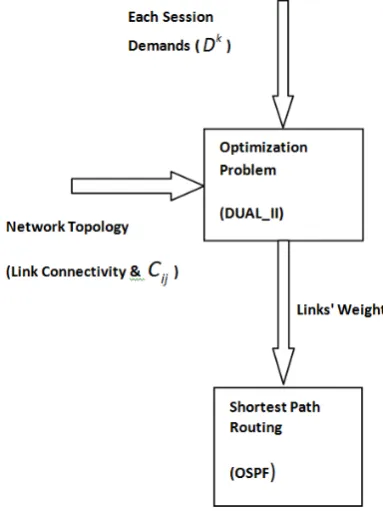
So we in this way, we were able to obtain optimal weights that do not include any link with weight 0 by limiting the constraint wij≥0 to wij′ ≥1. This converts the problem DUAL_TEMP to DUAL_II. Figure 1 shows the flow chart of our method.
With ECMP routing a flow arriving at a node is split evenly over the links on the shortest paths from this node to the destination. It should be mentioned that arbitrary routing is not possible once ECMP in OSPF is used. so in OSPF environment we can never obtain the optimal routing but we can get close to it as much as possible.
Objective function that is used in [8] is min
. The second term in this ob-jective function cause to minimizes
( , ) k ij i j A
X
∈
∑
in addi-tion to MLU. In this case the weight set resulted from the dual function is{
wij+r}
(where{ }
( , )
ij i j A
w ∈ are Lagrange multipliers that correspond to the non-equal constraint). The routing algorithm that we use in this paper is OSPF. This protocol splits the traffic equally among the available shortest paths, so we prefer traffic splitting as much as possible even if it passes through longer paths. As the constant
r
in the second term pre-vents the flow to go through long paths we assume that [image:4.595.75.267.464.720.2]0 r= .
Figure 1. Maximum load balancing flow chart.
5. Simulation Results
In this section we simulate the OSPF protocol with its default link metrics and with the metrics that are calcu-lated using the optimization problem.
A. Scenario I : In first scenario the simulation platform is shown in Figure 2.
All links in this network are DS3 with 44.7 Mbps rate. We suppose FIFO as a queuing policy. The session is a VOIP with GSM quality and the average bit rate is 40 Mbps. Node 1 is the source node and node 2 is the desti-nation.
Table 1 show the solution of primal problem ( ) which indicate the paths that minimize maximum utiliza-tion. Solution of DUAL_I problem is shown in Table 2 and Table 3 show the solution of DUAL_II problem.
Figure 2. Simulation network topology. Table 1. Optimum flows.
X12 20 X13 20 X23 0 X24 20 X25 0 X35 20 X54 20
Table 2. The Solution of DUAL_I.
[image:4.595.399.450.632.736.2]w12 0.0056 w13 0.0017 w23 0 w24 0.0056 w25 0 w35 0.0077 w54 0.0017
Table 3. The Solution of DUAL_II.
Table 1 show that the optimum paths are 1->2->4 and 1->3->5. These paths can obtain in a shortest path algo-rithm regarding to the weights that show in Table 2. Ta-ble 2 and Table 3 are the equivalent weights with respect to the graph that shows in Figure 2. So we use the sub-optimal weigh set in Table 3 instead of default OSPF link metrics. Figure 3 show that in recent method packet drop decrease significantly.
In fowlloing scenarioes (senario 2-) the simulation platform is shown in Figure 4. We compare MLU, BWE (Bandwidth Efficiency), Number of Over Utilized Links, IP Traffic Dropped and IP Traffic Received for all scena-rios
Figure.3. Dropping traffic in scenario1 for default protocol and new method.
Figure 4. Simulation Network Topology.
In fowlloing scenarioes (senario 2-) the simulation platform is shown in Figure 4. We compare MLU, BWE (Bandwidth Efficiency), Number of Over Utilized Links, IP Traffic Dropped and IP Traffic Received for all scena-rios
Scenario 2: In this scenario R1 is the traffic source and R13 is the traffic destination. Table 4 and Table 5 show the Suboptimal Link Weights that obtin by DUAL_II .
MLU in new method decreases from 91.3 percent to 36.3 percent and BWE increases from 7.6 percent to 10 percent as shown in Table 6.
Table 4. Solution of DUAL_II for Senario2.
W1_2 56.84 W3_6 1.000
W2_1 55.56 W6_3 1.000
W1_3 1.000 W3_7 1.000
W3_1 1.000 W7_3 1.000
W1_4 1.000 W4_9 1.000
W4_1 1.000 W9_4 1.000
W2_5 1.000 W4_8 1.000
W5_2 1.000 W8_4 1.000
W2_11 1.000 W5_12 1.000
W11_2 1.000 W12_5 1.000
W2_3 1.000 W6_11 1.000
W3_2 1.000 W11_6 1.000
W3_4 2.000 W6_10 1.000
W4_3 1.000 W10_6 1.000
Table.5. Solution of DUAL_II, cont for Senario2.
W6_7 55.84 W10_13 1.000
W7_6 1.000 W13_10 1.000
W7_10 1.000 W10_14 1.000
W10_7 1.000 W14_10 1.000
W7_9 1.283 W11_12 1.000
W9_7 1.000 W12_11 1.000
W8_9 1.000 W11_13 1.000
W9_8 1.000 W13_11 1.000
W9_10 1.000 W12_13 1.000
W10_9 1.000 W13_12 1.000
W9_15 2.000 W13_14 1.000
W15_9 1.000 W14_13 1.000
W10_11 1.000 W14_15 1.000
W11_10 1.000 W15_14 1.000
Table 6. MLU and BWE values for Senario2.
Default Algorithm
Suboptimal Algorithm MLU 91.3 36.3
BWE 7.6 10
Number of Over Utilized Link
IP Traffic Dropped and IP traffic Received do not change in this scenario because there is no congestion
[image:6.595.311.536.81.309.2]Scenario 3: in this scenario we have three source-des- tination pairs( ,s d1 1), ( ,s d2 2), ( ,s d3 3) that are origi-nated from R1 to R13, R5 to R9 and R4 to R2 respec-tively. MLU in the new method decreases from 137 per-cent to 91.3. The Number of over-utilized links also de-creases from eight links to two links. BWE inde-creases from 26.6 percent to 31.4 percent, Table 7. Figure 5 and Figure 6 show the comparison of IP Traffic Dropped and IP Traffic Received
6. Conclusion
[image:6.595.56.291.383.702.2]In this paper we show that Optimization Theory can help Internet protocols work better. We use a duality theory to find a weight set that improve the routing protocols effi-ciencies. As a matter of fact routing is the most important aspect of Internet Traffic Engineering. So we focus on routing protocols and introduce a practical method that optimizes Link Metrics. Previous optimization methods suffer from practical issues but our method could be im-plemented with Routing Protocols that based on
Table 7. MLU and BWE values for Senario 3.
Default Algorithm
Suboptimal Algorithm
MLU 137 91.3
BWE 29.6 31.4
Number of Over
Utilized Link 8 2
Figure 5. Ssenario2 IP traffic dropped.
Figure 6. Ssenario2’s IP traffic received.
shortest paths. Our simulation results show significant improvement on network efficiency.
REFERENCES
[1] Y. Lee et al., “Traffic Engineering in Next-Generation Optical Networks,” IEEE Commun. Surveys & Tutorials, vol. 6, no. 3, 2004, pp. 16–33.
[2] D. Awduche et al, “Requirements on Traffic Engineering over. 2. MPLS,” RFC 2702, June 1999.
[3] D. Awduche et al., “MPLS and Traffic Engineering in IP Networks, IEEE Commun. Mag., vol. 37, no. 12, Dec. 1999, pp. 42–47.
[4] B. Fortz et al., “Internet Traffic Engineering by Optimis-ing OSPF Weights,” Proc. IEEE INFOCOM, 2000, pp. 519–28.
[5] N. Hu et al., “Locating Internet Bottlenecks: Algorithms, Measure-ments and Implications,” Proc. ACM SIG-COMM, 2004, pp. 41–54.
[6] A.Marija et al “Two Phase Load balance Routing using OSPF,” IEEE JOURNAL ON SELECTED AREAS IN COMMUNICATIONS, VOL. 28, NO. 1, JANUARY 2010
[7] E. Oki et al” Load-Balanced IP Routing Scheme Based on Shortest Paths in Hose Model” IEEE Transaction on comminications, Volume : 58, Page(s): 2088 - 2096, 2010 [8] Z. Wang, Y. Wang, and L. Zhang, ”Internet Traffic Engi-neering without Full Mesh Overlaying,” INFOCOM’2001 [9] S. Boyd and L. Vanderberghe. Convex Optimization.
Cambridge Univ. Press, 2004