Stochastic Approximation Method for Fixed Point Problems

Stochastic Approximation Method for Fixed Point

Problems

Ya. I. Alber1, C. E. Chidume2, Jinlu Li3

1_{Department of Mathematics, The Technion-Israel Institute of Technology, Haifa, Israel} 2_{The Abdus Salam International Centre for Theoretical Physics, Trieste, Italy} 3_{Department of Mathematical Sciences, Shawnee State University, Portsmouth, USA}

Email: [email protected], [email protected]

Received August 28, 2012; revised November 28, 2012; accepted December 5, 2012

ABSTRACT

We study iterative processes of stochastic approximation for finding fixed points of weakly contractive and nonexpan- sive operators in Hilbert spaces under the condition that operators are given with random errors. We prove mean square convergence and convergence almost sure (a.s.) of iterative approximations and establish both asymptotic and nonasymptotic estimates of the convergence rate in degenerate and non-degenerate cases. Previously the stochastic ap- proximation algorithms were studied mainly for optimization problems.

Keywords: Hilbert Spaces; Stochastic Approximation Algorithm; Weakly Contractive Operators; Nonexpansive

Operators; Fixed Points; Convergence in Mean Square; Convergence Almost Sure (a.s.); Nonasymptotic Estimates of Convergence Rate

1. Introduction

In this paper the following problem is solved: To find a fixed point x of the operator in other

words, to find a solution

:

T GH, xG of the equation

,

xTx (1.1)

where T is a Lipschitz continuous mapping, H is a

Hilbert space, is a closed convex subset. We suppose that

GH

x exists, i.e., the fixed point set of

is nonempty. Note in different particular cases of the Equation (1.1), for example, when T G the

solution existence and solution uniqueness can be proved under some additional assumptions.

N

: G,

T



We separately consider two classes of mappings T: the

class of weakly contractive maps and more general class of nonexpansive ones. Let us recall their definitions.

Definition 1.1. A mapping is said to be

weakly contractive of class _{ t} on a closed convex subset if there exists a continuous and increas- ing function

:

T GH

C_

GH

 

t

 defined on IR such that  is po- sitive on IR

   

0 , 0 0,limt

 

t ,



and for all



, ,



.

x yG Tx Ty  x y  xy (1.2)

Remark 1.2. It follows from (1.2) that 

 

t

Definition 1.3. A mapping is said to be

nonexpansive on the closed convex subset if for all

:

T GH

GH

,

x yG

.

Tx Ty  xy

It is obvious that the class of weakly contractive maps is contained in the class of nonexpansive maps because the right-hand side of (1.2) is estimated as





0 x y  xy  x y , (1.3) and it contains the class of strongly contractive maps because 

  

t  1 q



t with 0 q 1 gives us

.

Tx Ty q xy (1.4)

We study the following algorithm of stochastic appro- ximation:





1 , 1, 2, , 1

n G n n n n ,

x_ Pr x  S x n  x G (1.5)

where PrG is the metric projection operator from H

onto G and deterministic step-parameters n satisfy the

standard conditions:

2

1 1

and .

n

n n

 

 

  n

 





  (1.6)

t

 and in real problems an argument of the function t 

 

t

doesn’t necessary approaches to  obeying the con- dition T G: H (see the example in Remark 3.4).

The factor _{n n} in (1.5) is an infinite-dimensional vector of random observations of the clearance operator

S x

F I T at random points x_nG



, ,

given for all on the same probability space

1

n



.

A P

,

n n n n

S x   (1.7)

where n xnTxn and n is a sequence of indepen-

dent random vectors with the conditions

 

2

1 1

0 and , 0 .

n n

E   E_ _C C   (1.8)

Here is a symbol of the mathematical expectation. In order to calculate conditional mathematical expecta- tions of different random variables we define the

E

 - subalgebra An:



x x1, , ,2  xn



on



, ,A P



. And then



_{n n}



means _n function with the following property: for any

E  A A-measurabl

n BA

e

 





 

d d

n n n

B B

P E A P .

   







We also assume in the sequel that n is An-mea-

surable for all n1.

Let us recall the mean square convergence and almost sure (a.s.) convergence.

We say that the sequence

 

_n of random variables

 

n

  converges in mean square to  if  exists and

2

lim n 0.

nE  

 _ _

 

The sequence n converges to  almost surely or

with probability 1 if

 

 



lim n



1.

n

P    

  

Almost sure convergence and convergence in mean square imply convergence in the sense of probability: The sequence

 

n of random variables  n

 

 

con-

verges in the sense of probability to   if for all

0



   





lim n 0.

nP      

So, we consider iterative processes of stochastic approximation in the form (1.5) for finding fixed points of weakly contractive (Definition 1.1) and nonexpansive (Definition 1.3) mappings in Hilbert spaces under the conditions (1.8). We prove mean square convergence and convergence almost sure of iterative approximations and establish both asymptotic and nonasymptotic estimates of the convergence rate. Perhaps, we present here the first results of this sort for fixed point problems. Formerly the stochastic approximation methods were studied mainly to find minimal and maximal points in optimization problems (see, for example, [1-6] and references within).

2. Auxiliary Recurrent Inequalities

Lemma 2.1. [3,4] Let

   

k , k and

 

k





1 1 , 1

k k k k k

      , 2, (2.1)

Assume that

1 k

k







 



and Then

1

. k k







 



 

k

is bounded and converges to some limit.

Lemma 2.2. [3,4] Let

     

k , k , k and

 

k be sequences of nonnegative real numbers satisfying the recurrent inequality.





 

1 1 ,

k k k k k k k

         1, 2, , (2.2)

where

1 1

,

k k

k k

 

 

 

  





 and either

1

k k







 



or

lim k 0.

k k  

  (2.3)

Assume that 

 

t

IR

is continuous and increasing func- tion defined on  _{such that  is positive on}

 

IR 0 , 

 

0 0. Then limkk 0. There exists

an infinite subsequence

 

k_l ,l1,2,, such that

1 0

1

1 l _,

l l

l

k

k k

k k k

C 

 

 





 

 

 

 

 

 







where 0





1

1 k .

k

C 











In the following two lemmas we want to present non- asymptotic estimates for the whole sequence k,k1.

For this the stronger requirements are made of para- meters k and function in the recurrent in-

equality.

 

t 

Suppose that 

 

t such that 

 

k _k, F t

 

and

 

t

 are antiderivatives from 

 

t and

 

1 _,

t

 re-

spectively, with arbitrary constants (without loss of generality, one can put

C

0

C ), i.e.

 

 

d ,

 

d

 

t .

F t t t t

t









 



Observe that F t

 

has the following properties:

i) F t

 



 

t ;

ii) F t

 

is strictly increasing on



1,



and

 

F t   as t ;

iii) The function

 

 

 

 

 

 be se- quences of nonnegative real numbers satisfying the re- current inequality.

t F

g t t

F t F t



   is decreasing;

iv) G t

 

lnF t

 

  as t .

Introduce the following denotations:

1) _1

 

_{z and }1

 

_{z are the inverse functions to}

 

t

 and 

 

t , respectively;

2)

 













0 1

0 1

1 , 2, 1

1

c s

v s s s c

s 

  

 





     



 

fixed control parameter;

3)



_,



1

 



 

 

₂



u s C   _ C a F s F _,

0 0

1

0, c 1;

C a

c



  

4) _{w s v r}



_,

 



_{ }1_



_{v r}

 



_{a F s}



 

_F

 



 2 ,

2  r ;

5)

 

1

 



 

₂

 

₁



Q c   _ c a F F _, where

0

c is an arbitrary fixed number;

We present now the based condition (P): The graphs

of the scalar functions and with any fixed are intersected on the interval

 

v s w s v r



,

 





2,



r 



2,



not more than at two points s1 and s2 (we do not con- sider contact points as intersection ones excepting s2

if any).

For example, the graphs of the functions v s

 

and

 



,

w s v r



calculated for

 

s b,b 0, 0 1 s

     ,

,

and 

 

t t, 1 satisfy the condition (P).

Lemma 2.3. [3,4] Assume that 1) the property (P) is carried out for the function



 

2



u s v



, 2

 



and

2) as

,

w s v

 

v s ; u s v



, 2

 



v s

 

s ; 3) the control ameter

.

 (2.4)

Then for the sequence

par c₀ is chosen such that

 



, 2



 

u s v v s ass 2

 

k generated by the in- eq

, (2.5)

it follows: uality

 

1 , 1, 2,

k k k k k k

       

limkk 0 and for all

. (2.6)

Lemma 2.4. [3,4] Assume that 1) the proper ca

1

k



,



, 1

 

,

k u k C C v

  max



Q



 2





ty (P) is rried out for all the function w s v



, 2

 

r



and v s

 

;

2) u s v



, 2

 



v s

 

as s . he seq



k



generated by the inequali Then for tty (2.5) limkkuence0.

dition,

a) if Q



In ad

  

1 v 2

 

uch that u s

and the control parameter is chosen s

(2.7)

b) in all remaining cases

0

c

 



 

, 2v v s as s2, then for

all 2k



 

;

k v k

 



,



,



   

1



u k C C

  max , 2 ,

1 ,

k Q v

k s





  (2.8)

 

, ,

k v k k s

   (2.9)

where is a unique root of the equation



,

  

u s C v s (2.10)

on the interval

s



2,



. g The followin re

lemmas deal with another sort of current inequalities:

Lemma 2.5. [7,8] Let

     

k , k , k and

 

k real numbers satisfying

be sequences of non-negative the recurrence inequality.

1

k k k k k,k 1, 2,

_      . (2.11) Assume that

1 1

and .

k k

k k

 

 

 

  







Then:

e exists an infinite subsequence

i) Ther

 

 

k k

  

such that

1

1 _,

k k

j j





 



  (2.12)

and, consequently, limkk 0; 0

ii) if limkk  and there exists  0 such that

1

k k k

    (2.13)

for all k1, then limkk 0.

] Let

Lemma 2.6. [7,8

     

_k , _k , _k and

 

_k

real numbers satisfying be sequences of non-negative the recurrence inequality (2.11). Assume that 



1

k k

 



and (2.3) is satisfied. Then there exists an infinite sub- sequence

 

_k 

 

k such that limkk 0.

3. Mean Square Convergence of Stochastic

Approximations

eorem 3.1. Assume

Th that T G: H is a weakly ss C_{ },

contractive mapping of the cla _{ }  1

 

 

 

is a convex function with respect to t2 and

2

1 .

E_ x x _  Then the sequence



xn



generated by (1.5)-(1.7) converges in mean square to a unique fixed point x of T. There exists an infinite subsequence

 

nl ,l1, 2,, such that

2 ₁

0 1

1 1

, 2

l l l

n n n

n n

E x x C C



 



 

 

 _ _{   }

 

   

 







(3.1)

where

 

2

 

1

   

the inequality

and some positive constant

(3.2) 0

C

satisfies



2



0 1

1 8 n .

n

C







 

Remark 3.2. exists in view condition in (1.6

no on

0

1C  

).

of the second

Proof. First of all, we te that the method (1.5)-(1.7)

guarantees inclusi xn G for all n1. Since the

metric projection 

operator PrG is nonexpansive in a

Hilbert space and xG exists, we can write





















2 1

2

n

x x



 

2

1 2

2 1

2 ,

2 ,

2 , .

G n n n n n G

n n n n n

n n n n

n n n n n

Pr x x Tx Pr x

x x x x

x x x x

x x x x

 

  

   

 



 

 

    

    

   

   

(3.3)

Let us evaluate the first scalar product in (3.3). We have





























2 2 2

1

,

n n n

x Tx x x

,

,

n n n

n n n

n n n

n n n n

n n n

x x Tx Tx x x x x Tx Tx x x x x Tx Tx x x

x x x x x x x x

x x x x x x



 

  

  

  

   

  

   

    

    

      

    

(3.4)

We remember that



 



 

2

 

1 .

   

(3.4) yield

Then the in- equalities (3.3) and









2 2

1

n n

x x  x x x

2

2 2

2

2 , .

n n

n n n n n n

x x x

 

    







   

(3.5)

Applying the conditional expectation with respect to

n

A to the both sides of (3.5) we obtain









2 1

n n

E x_ x A 

 _  _

 

2 2

2 2

2

2 , .

n n n

n n n n n n n n

x x x x

E x x A E A

 

    

 



   

 

 

 _  _ _  _

(3.6)

It is easy to see that

2 2

n n

 

  2

2 2

2 2

2 2 .

n

n n n n

n n n

E A

E A E A

E A

 

 

 

 

 

 

 _{ } _{ }

 

  _{ }

(3.7)

Since is weakly contractive and therefore non- expansive, one gets

T

2 2

4 .

n n n

x Tx  x x

Taking into account (3.7), the inequali mated as follows:

ty (3.9) is esti-













2

2 2

2

2 , 2 .

n n

n n

n n n n n n n

E x x A

x x x

E x x A E A

 

  

 

 



 

 

 

 

 

 _  _ _{ }

(3.8)

1

2 2

2

1 8n xn

 

 

  



Now the unconditional expectation implies













2 1

2 2

2

2 2

1 8 2

2 , 2

n

n n n n

n n n n n

E x x

E x x E x x

E x x E

  

   

 

 



 

 _  _

 

 

 

  _  _ _  _

   

 

 

 _  _ _{ }

(3.9)

Next we need the Jensen inequality for a convex fun- ction 



xn x 2



:







2



2

n n

E__ x x ___E_ x x __

(see [9,10]). This allows us to rewrite (3.9) in the form





2 1

n

E x_ x 

 _  _

 

2 2

2 ₂ 2

1 8

2 2

n n

n n n n

E x x

E x x E



   





 

  _  _

 

    

 _{ }  _ _{ }

 

 

(3.10)

because of



n, n



0

E_ x x _ .

Denoting n E xn x 2 

 

 _  _

  we have



2



 

2

1 1 8 2 2 1 ,

n n n n n C n

_           (3.11)

ew of Definition 1.1,

where in vi  

 

 

0 0

  is a continuous

ng function with . Due to (6), from Lemma 2.2 it follows

and increasi

2

lim n _0

n E x x

 

 _ 



and the estimate (3.1) holds too. The theorem is p

□

of we it is un ample wa

roved.

Remark 3.3. If a fixed point akly contractive mapping T G: H exists, then ique [11].

Remark 3.4. The following ex s presented in

[11]: Let Txsin ,x

 

0,1

t

G and It has been show

: .

3 1 sin sin

8

x y   x y xy

for all 0  x y 1. Then

 

3

 

4

 

2

1

1 _, 1 _and 1 _.

8 t 8t

         

8

que fixe

Definition 3.5. Let a nonexpansive mapping

:

T GH have a uni d point x. d c in

T is ve on the close onvex subset if there exists continuous and creasing func- said to be weakly sub-contracti

GH

tion 

 

t defined on IR such that  is positive on

 

0

IR , 

 

0 0,

tlim

 

t  , such that for all

xG.



2



,

x Tx x x  xx . (3.12)

Theorem 3.6. Assume that a mapping T G: H is weakly sub-contractive and the function 

 

t in (3.12) is convex on IR Then the results of Theorem 3.1 holds for the sequence

 

xn g erated by (1.5 (1.7).

Th u ) can

en

e second .6

assume n t less than linear growth )

ineq ality in (1 be omitted if we

o of  

 

“on in-

finity” and put n0

Assume

as

Theorem 3.7. tha ing is

weakly sub-contractive and the function is convex

n 

t a mapp T G: H



t





in (3.12) on IR Suppose that instead e conditions

1

lim n 0 and n .

n

  







  (3.13) 

of (1.6) th

n

hold. In addition, let n  0.5 and

 

lim 4 .

 

 

  14)

Then the sequence

 

_n

(3.

x generated by (1.5), (1.7) and

(3.13) converges in mean square to x. There exists an

infinite subsequence

 

n_l ,l1, 2,, such that

2 _{1 3}

1

1 _.

2 2

l l

n

E x x



 

 

 l

n n

n n

C 



 

 

 _{  }

  

 







where









2 2

1 1

,

2 8 ,

4 .

C

C

  

   

 



 

3.15)

Proof. Consider the inequality ( 11) in the for

,

n

2

3 1 1 2

2 1

2 8 max ,

C C x x C

C 



 

  

  (

m

 

2 2

1 2 2 1 8

n n n n C n n

_          

where n E xn x 2 .



 

 _  _

  Observe that it is derived by making use of (3.4) and the nonexpansivity property of

We shall show that .

T _n are bounded for all



1, 2,



.

n I  Indeed, since  

 

oncl is a us function, ude that

convex in- creasing continuo we c

 

 

1

   



 is nondecreasing and since (3.14) holds,

the inequality  

 

C14 has a solution

where  is the unique root of the scalar equ0

,

  _

(3.16)

ation  

 

C14. Together with this, (3.4) and

(3.14) are co-ordinated by the parameter  0.5. Only one alternative can happen for each nI:

er eith

 

2 2

1: 2 n n 2 1 n 8 n n 0

H       C    

or

 

2 2

1 2  n n 2 

2: n 8 n n 0.

H    C    

Den te o I1



nI H1is true



and





2 2is true

I  nI H . It is clear that I₁I₂I. From

the hypothesis H₁, it arises

 

n C1 4 n,

    

for all nI1. From the hypothesis and then n

2,

H we have: _n1_n for all nI₂. Consider all

1)

the possible cases:

2 .

I   Then _n_ for all nI.

2) I1 . Then n1 for all nI.

3) Let I1



1, 2,,N0



and I2



N01,N02,



.

Then n for n1, 2, , N0. By (3.16), 2

n C

0 1 2.

N C

 _  It is obvious that   for 0 2, 0 3, .

N  N   Therefore, _nC₂ for all nI.

4) Let I2 



1, 2, , N0



and I1



N01,N02,



.

Then n1 for n1, 2,,N0. and n for

0 1,N0 2,

N    Thus, _n_ fo I.

5) Let 1

r all n

I and I₂ be unbounded sets. Consider an

arbitrary interval



1, s 1



2,

s s 1

I n n_ I

where 1 I s1

   

.

, , 1,3,5,

s s

n n    It is easy to be sure that

s

n

 _ and nC2 for all nIs.

nded a

6) The other situations of bou nd unbounded sets 1

I and I₂

e th

are covered by ms 1)-5). Consequently

v e result: ll

the ite ,

we ha final n max



1,C2



for a .

nI

Thus, we obtain the inequality

 

2

1 2 3 ,

n n n n C n

_        (3.17)

where is defined by (3.15). Now Lemma 2.2 with n (2.3) implies the re

Rema . For a nction

3

C

ditio

the con sult. □

is convex and concave at the same time we suppose

2 c 4 .

Remark 3.9. If G is bounded or more generally

 

xn dif

is bounded, t e inequality (3.17) (with some ly follows from (3.16).

4. Estimates of the Mean Square

ble to gi

hen th ferent constant C3) immediate

Convergence Rate

Using Lemmas 2.3 and 2.4 we are a ve two general theorems on the nonasymptotic estimates of the mean square convergence rate for sequence

 

xn gene-

rat ti

(1.7)

re

ed by the stochas c approximation algorithm (1.5)- .

Again we introduce denotations 1)-5) from Section 2 induced now by the current inequality (3.11):

1) 1

 

z

 _and 1

 

z 

 are the invers

 

t

 and 

 

t , respectively;

2)

 

1



v s  C c s

e functions to

1

 is

, 



2





12C s1 ,c

 1 0  1 0

a fixed control parameter;

3)





1

 



 

 

2 2 2

, 2 0,

u s C   _ C a F s F



C 

0 1 ₁

c a

c



 

0

4)



_,

 



1



 





 

 

₂



_,

w s v r   _ v r a F s F _

; 2s,r 

5) 1







 

 



1 x a F 2 F 1 .

   

  _    _

 

ndition (P).

orem 4.1. Assume that all the conditions o Th are fulfiled and

i) the cond on (P) holds for the functions

and as

2

Q x

Introduce also the basic co

The f

eorem 3.1

iti

 



, 2





, 2

 



w s v u s v v s

 

;

ii) u s v



, 2

 



v s

 

s ;

iii) c₀1 is chosen such that u s v



, 2

 



v s

 

as

en the sequence 2.

 Th

s

 

xn generated by (1. )-(1.7)

co oint

5 nverges in average to a unique fixed p x of

an

T

d for all n1





0 , 2 ,

n

E_ x x _C u n C

 





, 2v





2 max .

C  Q

(4.1)

orem 4.2. Assu hat a he conditions of

Th m 3.1

i) th con s

2



 

The me t ll t

eore are fulfiled and

e dition (P) holds for the function v s

 

and w s v z



,

 



with any fixed z



2,



;

ii) u s v



, 2

 



v s

 

as s ;

iii) If and is chosen such that then the sequence

generated by (1.5)-(1.7) converges in average to a unique fixed point

 

2

Qv





v s

 

as

0 1

c 

2,

 

, 2

u s v s

 

xn

x of T and for all n1

 

2

0 ;

n

E_x x _C v n

 

iv) In all the remainin

(4.2)

g cases, (4.1) holds for 1 n s and (4.2) for ns, where s is a unique

of the eq

root uation u s C



, 2



v s





on the interval



2,



. u

Let s provide the examples of functions  

 

and

 

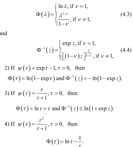
 [image:6.595.310.541.238.494.2]

 sui heorem and 4.2 (see [12,13]). 1) Below llaries 6 we use the functions

table for T s 4.1 in Coro 4.3-4.

 



   with  1. For them

 

1

ln , if 1,



 

  



 _{ }

, if 1, 1





 

  

(4.3)

and

 





1 , if 1,

if 1,

z

 



  

 1 (4.4)

1 exp

1 ,

z

z

 

  

 

 

 



2) If  

 

exp1, 0, then

 

_{ln 1 exp}





_and 1

 

_{ln 1 exp .}





z z

  

      

 

, 0

1



  



3) If   ,

 then

 

_{ln and} 1

 

_{ln 1 exp .}



z z

   

     



4)

 

2

, 0

1



  



If   ,

 then

 

 ln 1.



  

In this example we are unable to define _1

 

_z te it num

in an l form, therefore sugg lcula e- rically by computer.

We next present very important corollaries from The- or .1 and 4.2, where th ptions automatically guarantee accomplishment of the condition (P) (see [4]).

The functions

alitica est to ca

ems 4 eir assum

 

  .3. Ass

coincide with the point 1) a .

Corollary 4 ume that is a strongly

co ive mapping, that is satisfied with

.

bove

:

T GH

ntract ,(1.4) is

0 q 1 Let in (1.5) n ,b 0. n

 b  Then

 

 

1

 

1

1 1

ln

ln , , e ,q z 1 ,

t b t    z q q

q

F       

 

2 0 1 1





2 1

abq c C

v s     

1

1 2 1

1

1 _.

2

abq

b s s

Q x x

 

 _{   }

 

 

  _{ }

 

I. Suppose that 1

b q

 1 and 1

0 1

. 1

bq  Then bq c  2    lim

nEx 

1) If and

0

nx  and

 

2

Qv ₀ 1

1 , 2 bq c bq 

 we have for all

1 n

 

2 ; n

E_ x x _v n

  (4.5)

2) In all the remain cases





 





2

, ,

ma 2 , 1

n

E x x u n C

C Q n

  _ _        .6) and

x ,v s,

(4

 

2

, ,

n

x n s

 _ _{ }

 

  (4.7)

e

E x v s

wher s is a unique root of the equation



on the interval II. Suppose that



,

 

u s C v s



2,



.

1

2q ₁

1 1

b q

  and 1

0 1 1. 1 bq c bq   

Then lim n 2 0

n E x x

 

 _ _

 

 

r all n1.

and the estimate (4.6)

holds fo

Corollary 4.4. Assume that is a strongly

active mapping, that is, in (1.4) is satisfied with

. Let in (1.5)

:

T GH

contr

0 q 1 _n b ,b 0,0 1

n

     . Then

 

 

 

 













1 1 0 1 1 1 1 1 1 1 ln 1 , 1 2 2 2

2 1 .

1

b

q b

c C

v s C

b abq s ab               _        _    Suppose that 1 1 , ,

F t t

q  _       1 1 1 _,

z z q

  

 _  



2

, exp ,

1

u s C C

q      _ _      1 exp

Q x x 

1 , 1 s   0 . 1 bq c bq 

 Then

2

lim n 0

n E x x

   _ _     and

1) If Qv

 

2 and ₀ 1 1 , 2 bq c bq 

 we have for all

1 n

 

2 ; n

E_ x x _v n (4.8)

2) In all the remain cases the estimates (4.6) and (4.7) hold.

Corollary 4.5. Assume that is a weakly

contractive mapping of the class , that is, in Theorem 3.1

:

T GH

 t 2 1, 1

C_ t   

 

.

   Let in (1.5)

, 0

n

b b n

   . Then

 

 

  















  1 1 1 ₁ 1 1 1

2 2 1 1

1 1

ln , , 1 ,

1

1 1 ,

2

1 1

F t b t z z

C

x x x





1

, lns

u s C C ab

ln 2 .

Q x ab

          _            _  _       _     

If is chosen from the condition

 

 

  



   

01

c 1 1 0 1 1 2 2 c C C ab b  ,     _  _    

then lim 2 0

n E x x



 

n

    and for all n> 1



2



1

C c_{1 0} 

1 , ,

2

x , 2 .

n C Q C b ma C n

E_ x x _u

       _{  }  _       (4.9)

Corollary 4.6. Assume that is a weakly

contractive mapping of the class , that is, in Theorem 3.1

:

T GH

 t 2 1, 1

C_ t   

 

.

   Let in (1.5)

, 0,0 1

n b

b n

     . Then

 

 

  



 









 





1 1

1 1 ₁

1 0 1

1

1 1 1 1 ₂1 _,

u s b s

1 1

2 2 1 ₁

1 1

, , 1 ,

1 1 2 1 2 , 1 1 , 1 1 1 1 2 1 b

F t t z z

c C

v s C

b s

C C C a

Q x x x x ab

  _ 1 .           _           _              _  _           _{ }  _{ }              _  _         _    _   

I. Suppose that

1) If Qv

 

2 and c₀1 is chosen from the con-

dition

1



1 0 1

2 2

,

c C

ab b



 

1

2C

 

 

 

_{  }  _

_{ } 

 

 

then lim n 2 0

n E x x

 

 _ _

 

  and for all n1

 

2

.

n

E_ x x _v n

  (4.10) 2) In all the remain cases the estimates (4.6) and (4.7) hold.

II. Suppose that

1 _.

1

 

 

 



If c₀1 is chosen from the condition 1

1 0 1

1

2

2 ,

c C

C ab

b



 

 

 

 

_{  }  _

_{ } 

 

 

then lim 2

nE xn x 0



 _ _

 

  and for all n1









2





2

, , max , .

n

E_ x x _u n C C Q v

  (4.11)

In addition to the examples presented in this section, roduce the function

we p s  

 

and 







which have 0 as a tangency gree multiplicity and given logarithmic estimates of the con- vergence rate.

point of the infinite de

We define the function  

 

by the following way: 1



 

exp



f

 



f

 

, 0,

      _   _ 

where f

 

 is differentiable and decreasing function,

and

 

  , 0

limf 

 

 

 

 

_,

where

0

0 lim , 0,1, 2,

l l

l 

  

 

  

 

l  0

denote the derivative degrees o the function f

 

,

 

 

.

      It is easy to see that

 

 expf

 



  

and

 



 



1 _{z f} 1 _{ln z .}

 

  

In particular,

i)

 

1_,

 

2_exp 1 _.

f    

 



 

  We ha

 

 

  ve

1 exp





   and

 

 

1 _z 1 _.



  We have to

ln z

verify that  

 

is convex. In fact, it is true because

 

2

2

d 2 1 1

2 exp 0, 0.

d

   _

 



   

 

    

   

Beside this, it is easy to see that

   

 

,

   at least, on the interval

 

0,1

k these

. In the next eave to readers to chec properties.

examples we l

ii)

 

1 _{, 1,}

 

_exp 1 1_.

s s

s

f  s   

 

   _ _

 



 

We have

 

 exp 1_s



   and

 



 



1

1 _{ln s}

z



  z  .

iii)

 

_exp 1 _,

 

_exp 1 _exp 1 s1

s s

f    _s 

  



   

  __  _{ }

 

 

 

We have

 

 exp exp 1_s



 

   _{ }

  and

 



 



1

1 _{ln ln s.}

z z 



  

5. Almost Su

Approximations for Nonexpansive

ngs

Consider next the almost surely convergence of sto- chastic approximations. First of all, we need th sto- chastic analogy of Lemma 2.5:

re Convergence of Stochastic

Mappi

e

Lemma 5.1. Let

 

k be sequences of no -negative real numbers and

n

 

k be sequence of random Ak-

measurable variables, a.s. nonnegative for all Assume that

k

1.

k

1 1

an .

k k

k k

  

 

 

d

  







and there exists c0 such that for all If lim _k 0

k 

1

k





1 a.s.,

k E k An c k

 _     (5.1)

then lim _k 0

k  a.s.

The proof can be provided by the scheme of non-

[14] as ap ase of Hilbert spaces (the concepts of stochastic case (see Proposition 2 in [8]) or as it was done in [5].

We need also the following lemma from plied to our c

modulus of convexity  _B

 

of Banach spaces B or

Hilbert spaces H can be found in [15] and [16]). Lemma 5.2. If F I T with a nonexpansive mapping T G: H, then for all x y, D T

 

,





2

1

1

, ,

2

H

Fx Fy

  

Fx Fy x y R

R 

    

 



2 2



1

1 2 .

R   xy  Tx Ty  xy

If x R and y R with x y, D T

 

, then

 1 2

R R and



_,



1 2 _.

4

H

Fx Fy

Fx Fy x y L R

R 

   

    

 

eorem 5.3 that a mapping is

no

Th . Assume T G: H

nexpansive and its fixed point set N is nonempty. If

(1.8) holds and En An  C0, then the sequence

 

xn generated by (1.5)-(1.7) weakly almost surely converges to some xN.

Proof. Let xN. We next use Lemma 5.2 and the

estimate (see [17], p. 49)

 

2 8

H



  

to get





2 2

1

1 ,

2 32

H .

x Tx x Tx x Tx x x R

R



    

   _{ }

 

is case the inequality (3.3) implies In th





 





2 1

2 2

2 2 1

2 , 2 .

n

n n n n

n n n n n

x x

1 2

8 n x x 32 x Tx

x x

   







 

   



Similarly to (3.10), we have

  

 

 

(5.2)









2 1

2

n n

E x_ x A



 

 _  _

 

2 2

1 8n xn  Txn An

2 2

2nE n,xn x An 2nE n An .



2 n n

x Ex 

    _  _ (5.3)

 

 

 _  _ _{ }

Denote n E xn x 2 

 

 _  _ and _n E_ x_nTx_n 2

and apply the unconditional expectation to both sides of (5.3). Then

2 1 n





2



1 1 8 2 2 .

n n n n n C

          (5.4)

It follows from this that





1 1 8 2 1 .

n n n C n

2 2

_      

Since and due to Lemma 2.1, we con- clude that

2 1n 

 



 

n is bounded. Consequently,

 

xn is bounded a. ollows from the theory of co

quasimartingales (see [5,18]).

We now need Lemma 5.1. It is not difficult to see that

s. that f nvergent

2

1 1

.

n n nE xn Txn

  

 



 





_   _ (5.5)

The last gives us

2 1

a.s.

n xn Txn





  



Next we evaluate the following difference:









2 2

1 1

1 1

n n n n

x Tx x Tx

1 1

n n n

n n n n

x Tx x_n Tx

x Tx x Tx

 

 

 

   

It is easy to see that

 

   

 

n n

x Tx is bounded a.

si

s. Indeed, nce xn C₁ a.s., ther

ch that 2

0

C 

e exists a constant su

2

2 a. .

n n n

x Tx  x x C s

Therefore

1 1 2 2 a.s.

n n n n

x_ Tx_  x Tx  C

It is obviously that



 







1 1

1 1 2 1

Pr

2 2 .

n n n n

n n n n n n

n n n n G n

n n n n n

x Tx x Tx

x

2 PrG n

x Tx Tx x x

x Tx x

x Tx

 

  

 

  

   

     

  

  

Thus,

x

 





2 2

1 1

2

2 2

2 2 0

4 4

4 a.s..

n n n n n

n n n n

n

E x Tx A x Tx

C C E A

C C C

  



 

 

 _  _ 

 

  _{ }

 

By Lemma 5.1, xnTxn 0 a.s. as n .

Since

 

xn is bounded a.s., there is a subsequence

 

xnk weakly convergent to some point x. Sin

is convex a

ce closed, consequently, weak osed,

G

we

nd ly cl

assert that xG.

T

It is known that a nexpansi ng weakly demiclosed, there ore,

no f

ve

mappi is xN

quence a.s. Weak almost surely convergence of whole se

 

xn

Coro

is e standard way [8]. □ Assume that

co of the class If

shown

llary 5.

by th

4. T G: H is a weakly ntractive mapping C_{ t}.

1

,

n



  



2 1

n



  



and En An C₀, then the sequence

 

xn generated by (1.5)-(1.7) strongly almost surely erges to unique fixed point

conv x of

We have from (3.4)

.

T Proof.



2



.

n n n n

Since

 

xn is bounded a.s. and xnTxn 0 a.s. as we conclude that

,

n  



x_nx 2



0 a.s.

The proof follows due to the properties of the function

.

 □

s clear that all rema still va sel

case, e

t

Remark 5.5. It i the results in

lid for f-mappings T G: G. However, in this unlike any deterministic situation, th algorithm

(1.5)-(1.7) must use the projection operator PrG be-

cause the vec or vnxnnS xn n not always belongs to

G. If T xn nTxnnG for all n1 and

0n1, then (1.5) can be replaced by



1



, 1, 2,

1 1

n n n n n n , .

x   x  T x n  x G

S

[1] M. T. “Stochastic Approximation,” Cambridge Unive ss, Cambridge, 196

[2]

[3] “Nonasymptotic Estimates of the Convergence Rate of Stochastic Iterative Algori-thms,” Automation and Remote Control, Vol.

pp. 32-41.

[4] l Nonasymptoti

timate te of Iterative Stoc Algori nal Mathematics an



REFERENCE

Wasan,

rsity Pre 9.

M. B. Nevelson and R. Z. Hasminsky, “Stochastic Ap- proximation and Recursive Estimation,” AMS Providence, Rhode Island, 1973.

Ya. Alber and S. Shilman,

42, 1981, Ya. Alber and S. Shilman, “Genera c Es- s of the Convergence Ra hastic thms,” USSR Computatio d Ma- thematical Physics, Vol. 25, No. 2, 1985, pp. 13-20. doi:10.1016/0041-5553(85)90099-0

[5] K. Barty, J.-S. Roy and C. Strugarek, “Hilbert-Valued Perturbed Subgradient Algorithms,” Mathematics of Op- eration Research, Vol. 32, No. 3, 2007, pp. 551-562. doi:10.1287/moor.1070.0253

[6] X. Chen and H. White, “Asymptotic Properties of Some Projection-Based Robbins-Monro Procedures in a Hilbert Space,” Studies in Nonlinear Dynamics & Econometrics

/1558-3708.1000 Vol. 6, No. 1, 2002, pp. 1-53. doi:10.2202

[7] Ya. I. Alber and A. N. Iusem, “Extension of Subgradient Techniques for Nonsmooth Optimization in Banach Spaces,” Set-Valued Analysis, Vol. 9, No. 4, 2001, pp. 315-335. doi:10.1023/A:1012665832688

[8] Ya. Alber, A. Iusem and M. Solodov, “On the Projection Subgradient Method for Nonsmooth Convex Optimiza- tion in a Hilbert Space,” Mathematical Programming, Vol. 81, No. 1, 1998, pp. 23-35.

doi:10.1007/BF01584842

[9] A. P. Dempster, N. M. Laird and D. B. Rubin, “Maximal Likelihood from Incomplete Data via the EM Algorithm,” Journal of the Royal Statistical Society, Vol. 39, No. 1, 1977, pp. 185-197.

[10] W. Rudin, “Real and Complex Analysis,” McGraw-Hill,

98, 1997, pp. 7-

mimartingales,” De Gruyter, Berlin, 1982. New York, 1978.

[11] Ya. I. Alber and S. Guerre-Delabriere, “Principle of Weakly Contractive Maps in Hilbert Spaces,” Operator Theory, Advances and Applications, Vol.

22.

[12] Ya. I. Alber, “Recurrence Relations and Variational Ine- qualities,” Soviet Mathematics Doklady, Vol. 27, 1983, pp. 511-517.

[13] Ya. Alber, S. Guerre-Delabriere and L. Zelenko, “The Principle of Weakly Contractive Maps in Metric Spaces,” Communications on Applied Nonlinear Analysis, Vol. 5, No. 1, 1998, pp. 45-68.

[14] Ya. I. Alber, “New Results in Fixed Point Theory,” Pre- print, Haifa Technion, 2000.

[15] J. Diestel, “The Geometry of Banach Spaces,” Lecture Notes in Mathematics, No. 485, Springer, Berlin, 1975. [16] T. Figiel, “On the Moduli of Convexity and Smoothness,”

Studia Mathematica, Vol. 56, No. 2, 1976, pp. 121-155. [17] Ya. Alber and I. Ryazantseva, “Nonlinear Ill-Posed Prob-

lems of Monotone Type,” Springer, Berlin, 2006. [18] M. Métivier, “Se