Brownian Motion of Decaying Particles: Transition Probability, Computer Simulation, and First Passage Times

(1)

ISSN Online: 2153-120X ISSN Print: 2153-1196

DOI: 10.4236/jmp.2017.811108 Oct. 24, 2017 1809 Journal of Modern Physics

Brownian Motion of Decaying Particles:

Transition Probability

,

Computer Simulation

,

and First-Passage Times

M. P. Silverman

Department of Physics, Trinity College, Hartford, CT, USA

Abstract

Recent developments in the measurement of radioactive gases in passive dif-fusion motivate the analysis of Brownian motion of decaying particles, a sub-ject that has received little previous attention. This paper reports the deriva-tion and soluderiva-tion of equaderiva-tions comparable to the Fokker-Planck and Langevin equations for one-dimensional diffusion and decay of unstable particles. In marked contrast to the case of stable particles, the two equations are not equivalent, but provide different information regarding the same stochastic process. The differences arise because Brownian motion with particle decay is not a continuous process. The discontinuity is readily apparent in the computer-simulated trajectories of the Langevin equation that incorporate both a Wiener process for displacement fluctuations and a Bernoulli process for random decay. This paper also reports the derivation of the mean time of first passage of the decaying particle to absorbing boundaries. Here, too, ticle decay can lead to an outcome markedly different from that for stable par-ticles. In particular, the first-passage time of the decaying particle is always fi-nite, whereas the time for a stable particle to reach a single absorbing boun-dary is theoretically infinite due to the heavy tail of the inverse Gaussian den-sity. The methodology developed in this paper should prove useful in the in-vestigation of radioactive gases, aerosols of radioactive atoms, dust particles to which adhere radioactive ions, as well as diffusing gases and liquids of unsta-ble molecules.

Keywords

Brownian Motion, Random Walk, Diffusion, Radioactivity, Transition Probability, Fokker-Planck Equation, Langevin, Equation, First Passage, Fick’s Law, Wiener Process

How to cite this paper: Silverman, M.P. (2017) Brownian Motion of Decaying Par-ticles: Transition Probability, Computer Simulation, and First-Passage Times. Jour-nal of Modern Physics, 8, 1809-1849. https://doi.org/10.4236/jmp.2017.811108

Received: September 18, 2017 Accepted: October 21, 2017 Published: October 24, 2017

http://creativecommons.org/licenses/by/4.0/

(2)

DOI: 10.4236/jmp.2017.811108 1810 Journal of Modern Physics

1. Introduction: Two Approaches to Brownian Motion

Brownian motion, one of the simplest examples of a random walk, is a nonequi-librium statistical process the mathematics of which serves to model a wide va-riety of stochastic processes throughout the physical and social sciences. From the earliest applications of Einstein to the random motion of small particles in a fluid [1] and of Bachelier to price fluctuations of the stock market [2] up to the present day, diffusive processes have been investigated intensively and reported in numerous monographs, textbooks, and articles of which the following provide representative examples of methods and applications [3]-[9].

Despite their great diversity, nearly all such studies known to the author have in common the feature that the diffusing particles maintain their identity throughout the stochastic process. There are a few exceptions, such neutron dif-fusion with beta decay in reactor materials [10] [11] or the chemical transforma-tion of diffusing reactants leading to pattern formatransforma-tion [12] [13] [14], but the content and objectives of these investigations are very different from those of this paper, which was motivated by recent experimental studies of the diffusion of radioactive gases [15]. In contrast to previous treatments of diffusion, the subject matter of this paper concerns the transition probabilities, statistical mo-ments, and computer simulation of the Brownian motion of particles that can decay randomly. To underscore the distinction further, note that the decay terms that may appear in the equations of motion of well-studied stochastic processes such as the Ornstein-Uhlenbeck process [16] arise from the frictional interaction of a stable particle with the environment and involve only the process variables, like velocity, of the diffusing particle. In the Brownian motion treated in this

paper, there is no frictional interaction with the environment, and it is the dif-fusing particles themselves that decay.

Under the assumption, usually justified by the Fermi Golden Rule of time- dependent perturbation theory in quantum mechanics [17], that the probability of particle decay within a short time interval ∆t takes the form

( )

1

p ∆ = ∆t λ t ,

(1)

where

λ

is the intrinsic decay rate, it is readily deducible [18] that the proba-bility density of survival to time t satisfies the differential equation

( )

dp t dt= −λp t

(2) with normalized solution

( )

e t

p t =

λ

−λ . (3)

From Equation (3) it follows that the mean lifetime τ _{is the reciprocal of}

λ

( )

1

0tp t dt

τ

₌ ∞ ₌

λ

−

∫

,

(4) and that the half-life, i.e. duration within which the survival probability is 50%, is

1

1 2 ln 2 ln 2

(3)

The premise that the probability (1), with

λ

independent of environmental interactions, accurately characterizes the transmutation of radioactive nuclei has been challenged on various grounds during the past 20 years. However, in each case the theoretical consequences of relation (1) were validated experimentally and shown to be in accord with currently known laws of physics [19] [20].

Because unstable particles are removed from the system at random instances during the time they are moving randomly within a specified sample space, the familiar standard equations (e.g. Langevin and Fokker-Planck) for Brownian motion must be re-derived on the basis of a conservation law that takes particle loss into account. This more general relation, presented in Section 2, leads to significant differences in the analytical structure of the stochastic equations and statistical moments compared with corresponding expressions derived for the random walk of a stable particle.

In general, there are two mathematically different approaches to analyzing Brownian motion. One method, to be referred to as the Langevin approach, is to examine the process variables directly. For a particle undergoing a one-dimensional random walk, the process variable of interest in this paper is the displacement

( )

X t as a function of time t. Conventional symbolic notation, which is used in

this paper unless stated otherwise, employs an upper-case letter (e.g. X) to de-signate a random variable and a corresponding lower-case letter (e.g. x) to represent a realization or measurement of the variable (referred to as a variate in statistical terminology). The Langevin equation of motion for the time-evolution of the coordinate variable usually takes the form of an Ito stochastic differential equation [21]

( )

(

)

( )

(

)

(

)

( )

dX t ≡X t+dt −X t =A X t, dt+ B X t, dW t

(6) in which A X t

(

,

)

is the drift function, B X t

(

,

)

is the diffusivity, and

( )

dW t = dt N 0,1 is the differential Wiener process in which N

( )

0,1 sym-bolizes a Gaussian distribution of mean µ =0 and variance σ =2 1. The drift

(

,

)

A X t is a deterministic function, whereas the Wiener term is the source of

fluctuations.

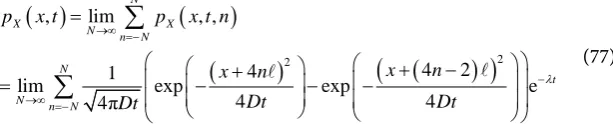
It is clear from Equation (6) that the analytical solution, if one can be found, is not a deterministic function of a dynamical variable, but a probability distribu-tion. A distribution is said to be stable if two independent random variables characterized by this distribution sum to form a random variable governed by a distribution of the same kind [22]. Gaussian and Lorentzian processes are stable, but most stochastic processes are not. For example, in regard to a Gaussian dis-tribution whose probability density function (PDF) takes the general form

(

)

(

)

2 2

)

2

1

, exp 2

2π

X

p xµ σ x µ σ

σ

= − − , (7)

one can express the corresponding random variable as

(

2

)

( )

, 0,1

X =N µ σ = +µ σN

(4)

and the sum of two independent Gaussian random variables as

(

)

(

) (

)

( )

2 2 2 2

1 2 1 1 1 2 2 2 1 2 1 2

2 2

1 2 1 2

, , ,

0,1 .

X X N N N

N

µ σ µ σ µ µ σ σ

µ µ σ σ

+ = + = + +

= + + +

(9)

It follows from the stability relation (9) that the solution to (6) is itself a Gaus-sian distribution.

The second method, to be referred to as the Fokker-Planck approach, is to solve for the transition probability function (TPF) p x t x t

(

, 0,0

)

of finding the particle at location x at time t, given that the particle was initially at x0 at time

0

t <t. The partial differential equation corresponding to the stochastic

differen-tial Equation (6) is the forward Fokker-Planck equation [Ref [3], pp. 117-122]

(

)

(

( )

(

)

2

(

( )

(

)

0 0 0 0

0 0

2

, , , , , ,

, , 1

2

A x t p x t x t B x t p x t x t

p x t x t

t x x

∂ ∂

∂

= − +

∂ ∂ ∂ . (10)

For non-decaying particles, Equations ((6) and (10)) have the same informa-tion content, but provide different perspectives on the same stochastic process. For example, the stochastic differential Equation (6) is particularly suitable for numerical solution by an iterative up-dating algorithm, thereby permitting computer simulation of particle displacement and visualization of the process variables in real time. On the other hand, the forward Fokker-Planck Equation (10) yields a probability density function from which all statistical moments can be calculated. The solution p x t x t

(

, 0,0

)

also solves the backward Fokker- Planck equation [Ref [8], pp. 168-171]

(

)

(

)

(

)

(

)

2

(

)

0 0 0 0 0 0

0 0 0 0 2

0 0 0

, , , , 1 , ,

, ,

2

p x t x t p x t x t p x t x t

A x t B x t

t x x

∂ ∂ ∂

= − −

∂ ∂ ∂ , (11)

in which derivatives are taken with respect to the initial coordinates. Equation (11) provides the same information as the forward Fokker-Planck Equation (10), but is of particular utility in the analysis of Brownian motion within a region confined by boundaries. The structure of Equation (11) facilitates treatment of the problem of first-passage times to be analyzed in Section 3 by alternative, simpler methods.

Generally speaking, one solves a Brownian motion problem to answer two kinds of questions: 1) How far has a particle randomly walked in a given time? and 2) In how much time will a particle randomly walk to a given location? It is to be understood, of course, that answers to questions like these are probabilistic, not deterministic, statements. Questions of the first kind are perhaps more fa-miliar, but there are numerous circumstances that call for answers to questions of the second kind. These are usually referred to as first-passage processes [23], and in statistical terminology the time to reach a designated location has been called first-passage time, first hitting time, first return time, exit time, and possi-bly other names depending on the exact circumstances.

(5)

with absorbing boundaries. Derivation and analysis of the equations corres-ponding to the Fokker-Planck equation and Langevin equation will show that these equations do not lead to equivalent descriptions of the Brownian motion of a decaying particle, in marked contrast to the case of stable particles. This ine-quivalence is traceable to the fact that particle decay is a discontinuous process. The Fokker-Planck equation, which yields a transition probability density, re-mains a continuous differential equation, but the Langevin equation, which de-scribes a process variable, and not a probability density, must directly manifest the discontinuous nature of decay.

The distinction between the Brownian motion of stable and unstable particles becomes very apparent in the problem of first-passage time to absorbing boun-daries. Upon reaching an absorbing boundary for the first (and therefore only) time, the particle is removed from the system and the process is terminated. Likewise, upon decay at some unpredictable moment, the particle is also re-moved and the process is terminated. Thus, the instability of the particle intro-duces into a first-passage problem an additional time element that can radically modify expectation values. From the perspective of physics, this modification extends the applicability of first-passage time theory to a broader class of physical systems. As a physical model, the solution to a first-passage time problem with particle decay has been applied to the diffusion of the radioactive gas radon-222 in the atmosphere, and should likewise prove useful in the study of diffusion of other radioactive gases, radioactive ions that form as daughter products in radioactive decay, as well as unstable molecules that change their identity by chemical transformation.

As a purely stochastic problem, the analysis undertaken in this paper

• derives and provides an exact solution to the Fokker-Planck and Langevin equations of Brownian motion of an unstable particle,

• _{extends to unstable particles the two principal methods of calculating}

first-passage times,

• _{demonstrates how to simulate by computer the Brownian motion of an}

un-stable particle, and

• _{clarifies a number of confusing issues that arise in the case of unstable}

par-ticles (but not stable parpar-ticles) regarding Fokker-Planck and Langevin equa-tions, expectation values, probability density funcequa-tions, and transition proba-bility functions.

(6)

Brownian motion trajectories of the decaying particle are given in Section 2.3. In Section 2.4 the Langevin equation is solved analytically to obtain the distribution function of the particle displacement. Section 3 is concerned with temporal as-pects of a decaying particle undergoing a one-dimensional random walk. The mean first-passage time to absorbing boundaries is solved in Section 3.1 by the method of image functions and in Section 3.2 by solution of a screened Poisson equation. Section 3.3 illustrates the critical role of particle decay in leading to first-passage time results that differ markedly from corresponding results for a stable particle. Section 4 examines the validity of the stochastic model, based on a Wiener process or Fick’s law, to account for fluctuations in the spatial dis-placement of a decaying particle. Finally, conclusions drawn from these analyses are summarized in Section 5.

2. Diffusion with Decay

2.1 Fokker-Planck Equation and Transition Probability

Consider a quantity

( )

, d V

Q t =

∫∫∫

n x t V of particles with decay constant

λ

and number density n

( )

x,t within a volume V bound by surface S. Since loss

of Q can occur either by intrinsic decay at the rate −λQ or by diffusion of a

current density j x

( )

,t outward across surface S, macroscopic mass balance

requires that

d d d

V S V

n V n V

t λ

∂ _{= −} _⋅ ₋

∂

∫∫∫



∫∫

j S

∫∫∫

. (12) Application of the divergence theorem then leads from the integral relation (12) to the differential equation

n

t λ

∂ _{= −∇ ⋅ −}

∂ j (13) for the conservation law of a disintegrating quantity.

Upon dividing Equation (13) by the initial number of particles N0 1 and relating the current density to the gradient of the particle density by Fick’s law

= − ∇D n

j , (14) with diffusion coefficient D (here taken to be a constant), one obtains an equa-tion of the form

2

w

D w w

t λ

∂ _{= ∇} ₋

∂ (15) in which w

( ) ( )

x,t =n x,t N0 is interpretable as the probability density for diffusion of a single decaying particle. However, it is demonstrable that the solu-tion w

( )

x,t under the special initial condition at t₀

(

,0

)

(

0

)

w x t =δ x−x

(7)

t given that it was at x0 at t0<t. The equivalence is readily established by substitution of condition (16) into the Chapman-Kolmogorov equation [24]

( )

(

)

(

)

(

)

(

)

(

)

1 0 1 0 1

1 0 1 0 1 0 0

, , , , d

, , d , , .

w t p t t w t

p t t

δ

p t t

∞ −∞ ∞ −∞ =

= − =

∫

x x x x x

x x x x x x x

(17)

In the case of one-dimensional Brownian motion treated in this paper, Equa-tion (15) then takes the form

(

)

2

(

)

(

)

0 0 0 0

0 0 2

, , , ,

, ,

p x t x t p x t x t

D p x t x t

t x λ

∂ ∂

= −

∂ ∂ , (18)

which, together with the initial delta-function condition (16)

(

, 0 0,0

)

(

0

)

p x t x t =δ x−x

(19) comprises the equation for the Green’s function of a one-dimensional random walk with decay [25].

The solution to Equations ((18) and (19)) can be obtained in several ways. One method is to take the Fourier transform with respect to the spatial coordi-nate, which converts the partial differential Equation (18) of two variables (space, time) into an ordinary differential equation in one variable (time). The simplest method, however, which has been used to solve the Schroedinger equation for transitions between excited atomic states [26] and the rate equations for a se-quence of nuclear transformations [27], is to eliminate the decay term in Equa-tion (18) by the substituEqua-tion p x t x t

(

, 0,0

)

=p0

(

x t x t, 0, 0

)

exp

(

−λ

(

t−t0

)

, the-reby transforming Equation (18) into the equation for the Green’s function

(

)

0 , 0,0

p x t x t of a non-decaying diffusing particle, the solution of which is

known [Ref [6], p. 12]. Either way, one obtains the transition probability func-tion (TPF)

(

)

(

)

(

)

(

)

( 0)

2

0 0 0 0

0

1

, , exp 4 e

4π

t t

p x t x t x x D t t

D t t

λ − −

= − − −

− .

(20)

From the form of relation (20), one sees that the transition probability is a function of the time interval t−t0, and not the separate time coordinates

( )

t t,0 . From this point on, it will be assumed that t0 =0 and t will represent a time interval.

Although the functions w x t

( )

, and p x t x

(

, ₀, 0

)

are mathematically iden-tical in form, they serve different purposes and are used to calculate different quantities. For example, the probability density function (PDF) is employed to calculate the statistical moments

{ }

mk of a distribution, where the

th

k

mo-ment (expectation value) with respect to the origin is defined by

( )

, d

( )

, d

k k

m =

∫

x w x t x

∫

w x t x, (21)

(8)

( )

, d

(

, 0

)

d e

t

w x t x p x t x x λ

∞ ∞ ₋

−∞ = −∞ =

∫

, (22)

but yields, instead, the survival probability to time t of the unstable particle. In contrast to (21), the TPF is employed to calculate transition probabilities and statistical moments of a different nature. For example, the expectation value of the th

k power of displacement of a particle in time interval t starting from

po-sition x0 is

(

0 0

)

, , 0 d e

k k t

k

x =

∫

x p x t x x=m −λ .

(23)

Because the TPF is a conditional probability, the expectation value (23) does not include a normalizing denominator as in Equation (21). For a stable particle, relations (21) and (23) yield the same result, but this is not the case for a decay-ing particle.

The distinction between PDF and TPF leads to different results for the mean- square displacement. Employing solution (20) as the Gaussian PDF w x t

( )

, in the expectation value (21), one obtains the meanlocation m1=x0 and variance

about the mean

2 2 1 2

m −m = Dt (24)

of a non-decaying diffusing particle. However, calculation of expectation values (23) with the TPF p x t x

(

, 0, 0

)

leads to the initiallocation x =x0 of the dif-fusing particle and its mean-square distance from the point of origin

( )

2

2 e t

x t Dt

λ

σ

₌ − _{. (25)}

Thus, the same mathematical function (20) generates expectation values that differ in interpretation and mathematical form depending on what is sought by the analyst. In the context of understanding how decay affects the probability of displacement of a single particle in continuous Brownian motion, relation (25) is the relevant quantity, as shown in the following section.

2.2. Mean-Square Displacement

Consider a one-dimensional Gaussian random walk on a lattice with time step

t

δ

and displacement

δ

Xj during the jth time step given by

( )

0,1

j j

X XN

δ =δ

(26) where the lattice spacing

δ

X sets the scale of spatial displacement. Each

dis-placement is taken to be an independent Gaussian random variable. However, a displacement can be made only if the particle has survived during that time step. From Equation (3) it is seen that the probability of survival during a time step

t

δ

is ps= −1 λδt, and the probability that the process ends at a particular

time step is

λδ

t. Thus, although the distance traveled in the jth time step is

de-termined by a unit normal distribution N_j

( )

0,1 , the probability that the dis-placement is made at all is determined by a Bernoulli random variable

(

1,

)

1 with probability 1

0 with probability 1

s j j s

s

p t

B p

p t

λδ ε

λδ = − 

= =  ₋ ₌

(9)

A Bernoulli distribution is the special case n=1 of the binomial distribution

(

,

)

B n p of n trials with probability of success p; the corresponding discrete

probability function is

(

)

(

)

(

)

B , 1 0

n k k

n

p k n p p p n k

k

−  

=_{ } − ≥ ≥

  . (28)

The subscript j in relations (26) and (27) denotes that each random sample, whether Gaussian or Bernoulli, is independent of all the others.

The displacement after n time steps is given by the random variable Xn

( )

1 1

0,1 0,

n n

n j j

j j

X δX δX N δX N n

= =

=

∑

=

∑

= _{. (29)}

The expectation value of the mean square displacement at time t=n t

δ

is

therefore

(

)

2

(

( )

)

2

(

) (

2

)

2 _0, n ₁ n

n s

X = δX N n p =n δX −λδt , (30)

which can be re-expressed in the form

( )

2 2

1

n n

X t

t n

δ

λ

δ

 _ _

 

= _ _ − _

 

  . (31) Upon defining the diffusion constant D in the standard way

( )

2 2D= δX δt

(32) and taking the limit

δ

t→0,

δ

X →0, with requirement that D remain finite,

Equation (31) becomes

2

2 e t t

X = Dt −λ

(33) in accord with the expectation value (25) obtained directly from the TPF (20).

As a point of clarification, the reason for the factor of 2 in the conventional definition (32) of the diffusion coefficient is that the quantity 2D corresponds

to the fluctuation function B x t

( )

, in the Wiener term of the forward Fokker- Planck Equation (10). Under the conditions that B x t

( )

, =2D is constant and

there is no drift, A x t

( )

, =0, Equation (10) then reduces to the standard one- dimensional diffusion equation

(

)

2

(

)

0 0 0 0

2

, , , ,

p x t x t p x t x t

D

t x

∂ ∂

=

∂ ∂ (34)

in which D is the physically measurable diffusion constant first introduced by Einstein in his theory of Brownian motion.

2.3. Langevin Equation: Update Algorithm

and Computer Simulation

The Langevin Equation (6) for one-dimensional Brownian motion of a non-decaying particle in the absence of drift is expressible in a form

(

d

) ( )

2 d t

x t+ t =x t + D tn

(10)

that facilitates numerical solution by an update algorithm. The lower-case letters

x in Equation (35) signify numerical realizations of the random variable X in Equation (6); dt is the numerical time step; and nt is a random sample from

the unit normal distribution d

( )

0,1

t t t

N+ , where the subscript t and superscript d

t+ t explicitly denote the temporal range with respect to which nt is

asso-ciated. Thus, two samples nt1 and nt2 , corresponding to distributions

( )

1 1 d

0,1 t t t

N + and 2

( )

2 d

0,1 t t t

N + , are independent for t2− >t1 dt. Given an initial value x

( )

0 , a sequence of points

{

x

( ) ( ) ( )

0 ,x d ,t x 2d ,t ,x n t

( )

d

}

is generated by iterative use of Equation (35) up to time t=n td . (Note: The symbol n

with-out subscript is the number of time steps, not a sample from a normal distribu-tion.) The sequence of points is an approximation to the true Brownian motion in the limit dt→0. In that theoretical limit, the trajectory of Brownian motion

is a curve that is everywhere continuous, but nowhere differentiable; in other words, a particle trajectory for which the particle velocity is undefined.

Although Equation (35) is simple enough to be solved analytically, a numeri-cal solution provides a graphinumeri-cal visualization of Brownian motion paths. More-over, starting from the same initial condition and generating numerous Brow-nian trajectories for a specified time interval t provides a Gibbs ensemble [28] [29], from which ensemble and time averages of moments, correlation functions, and other statistical quantities can be obtained by Monte Carlo methods [30] [31]. Such methods are particularly useful when the Langevin or Fokker-Planck equations cannot be solved analytically.

The question addressed in this section is this: What is the Langevin equation for Brownian motion of a decaying particle? Since the Langevin and Fokker- Planck equations of a stable particle ordinarily provide equivalent information, one can in principle start with either one and obtain the functions A x t

( )

, and

( )

,

B x t needed for the other. Thus, for a stable particle the Langevin Equation

(35) leads to the corresponding Fokker-Planck Equation (34), and vice-versa. It is to be stressed, however, that only a continuous Markov process is completely and equivalently defined by either the Langevin equation or Fokker-Planck equ-ation [Ref [8], p. 158]. In the case of a decaying particle, the Brownian motion is not a continuous process because it is abruptly terminated by disintegration of the particle. Equation (18)—although referred to in this paper as a Fokker- Planck equation in deference to conventional usage—is actually not in the form of a Fokker-Planck equation. The term λp x t x t

(

, 0,0

)

is not a drift term since it does not involve the spatial derivative of p x t x t

(

, 0, 0

)

. Here, then, is another important difference in the Brownian motion of a particle that decays randomly compared to one that is stable.

Theoretically, it is possible to transform Equation (18) into a Fokker-Planck equation. One merely needs to find a drift function A x t

( )

, that satisfies the differential equation

( )

(

)

(

A x t p x t x t, , 0,0

)

p x t x t

(

, 0,0

)

x

λ ∂ =λ

(11)

Integration of Equation (36) yields

( )

, π erf exp 2

4 4

x x

A x t Dt

Dt Dt

 

= _ _ _ _

   (37) with boundary and initial conditions

( )

0, 0,

( )

, 0

( )

A t = A x δ x . (38)

The error function is defined by the integral

( )

2

( )

0 2

erf e d erf

π x _u

x ≡

∫

− u= − −x .

(39)

However, the preceding solution (37)—or, indeed, any transformation that generates a Fokker-Planck equation from Equation (18) by finding a drift term—seriously misrepresents the physics of the problem. This is a stochastic process, as emphasized in the preceding sections, in which the physical particle (or the probability of particle existence), and not a process variable, is decaying. There is neither drift nor friction in this process.

The key point to recognize in constructing an appropriate stochastic differen-tial equation—which, for the sake of conventional nomenclature, is referred to in this paper as a Langevin equation, even though rigorously it is not—is that the unstable particle, as long as it exists, undergoes Brownian motion as described by the standard diffusion Equation (35). The Brownian motion does not contin-ue indefinitely, however, but is interrupted randomly by particle decay. The first instance of decay terminates the process; there is no further diffusion of that particle. (One could then introduce another particle and follow its Brownian motion if it is desired to acquire an ensemble of trajectories.) The stochastic process, therefore, entails sequences of two paired independent distributions: (a) the unit normal distribution d

( )

0,1

t t t

N+ , which determines the direction and

extent of displacement during the time period

[

t t, +dt

]

, and (b) the Bernoulli

distribution d

(

)

1,

t t

t s

B+ p , which determines whether or not the particle survives

the interval dt with a survival probability ps given by Equation (27).

The appropriate Langevin equation would then take the update form

(

d

)

( )

2 d _t _t

x t+ t =_x t + D tn_ε

(40) where the Bernoulli variate

ε

t is defined in relation (27). Note that an

occur-rence of ε =t 0 terminates the entire process by setting x t

(

+dt

)

to zero. Thus,

just before the moment of decay, the particle will have reached location x t

( )

and no further. Although the Langevin Equation (40) and the TPF Equation (18) both describe Brownian motion of a decaying particle, the descriptions are not equivalent. The TPF is a continuous probability function for all displacements x

of a given particle; there is no built-in mechanism to terminate the process at decay. The Langevin Equation (40) has such a mechanism.

(12)

( )

(

)

( )

(

)

( )

1 1

1 1 2 2 2

1 1 2 3 2 2 3 3 3

1 2 3

d 2 d

2d 2 d

3d 2 d

d 2 d .

n n n

j j j n n

j j j

x t D tn

x t D t n n

x t D t n n n

x n t D t n n n n

ε

ε ε ε

ε ε ε ε ε ε

ε ε ε ε

= = = = = + = + +   = _ + + + + _ 

∏

   (41)

The mean displacement x n t

( )

d =0 follows immediately from the proper-ties of the unit Gaussian t dt

( )

_0,1 ₀

t t

n = N+ = . The mean-square displacement

is less obvious and leads to two results depending on whether one retains the structure of discrete time steps or takes the limit for continuous displacement in time.

Consider first the continuous-time limit of the mean-square displacement, where one sets dt=t n and eventually takes the limit n→ ∞ and dt→0

such that t is a fixed quantity. Equation (41) then yields

( )

( ) ( )

2

2 2 2 2

2 2

1 2

d

2 n n

j j n n

j j

x n t

Dt

n n n

n = ε = ε ε

 

=  + + + 



∏

 

(42)

where the Bernoulli variates ε =t 1 at each time step (otherwise there would not

be n steps). There are no cross-terms in the expectation values because all the Gaussian and Bernoulli samples are realizations of independent uncorrelated random variables. Upon insertion in Equation (42) of the expectation values

( )

2 2 1 1 , t t s n t p n ε λ =   = = −_ _   (43)

summing the terms in Equation (42), and taking the forementioned limit, one arrives at

( )

(

)

2

1

2 2

1 1 e

j n

t n

j

Dt t D

x t n n λ λ λ − →∞ =   = _ − _ → −  

∑

. (44)

It should not be surprising that expression (44) differs from the mean-square displacement (25) derived from the TPF, because Equation (18) provides differ-ent information than the stochastic differdiffer-ential Equation (40). As shown in Sec-tion 2.2, the expectaSec-tion value (25) is equivalent to the mean-square displace-ment of a particle prior to decay multiplied by the survival probability to time t. Statistically, it may be thought of as a compound stochastic process N

( )

0,n ×

(

, _s

)

B n p . By comparison, one can think of the outcome (44) as resulting from a

sum of n compound stochastic processes of the form N

( )

0,1 ×B

(

1,p_s

)

.

It is of interest to examine the two limiting cases of Equation (44):

( )

(

)

2 2 1

2 1 Dt t x t D t λ λ λ  →   

(13)

The first limit in (45) shows that the mean-square displacement of a particle whose statistical lifetime is much longer than the diffusion time is the same as for Brownian motion of a stable particle. The second limit shows that the root- mean-square distance 2

( )

x t reached by a particle very likely to decay

dur-ing the diffusion time is equivalent, within a factor 2, to the characteristic

diffusion length [15]

D

ζ

=

λ

(46) that occurs in the solution of the diffusion equation for radioactive gases [32]. Recall, however, that 2D, rather than D, is the mathematical diffusivity

equivalent to the function B x t

( )

, appearing in the Fokker-Planck Equation (10). In this paper, therefore, the mathematical diffusion length will be defined as ζm≡ 2D λ.

Consider next the mean-square displacement as obtained from Equation (44) with n discrete time steps of duration

δ

t

( )

(

)

(

)

2

1

2

2 1 1 1

n

n j

s j

D

x n tδ D tδ p λδt λδt

λ =

 

=

∑

= − _ − − __{, (47)}

where use was made of the summation formula for a geometric series 1

1 0

1

1 1

1

n

n n

j j

p

p p

p

+

= =

−

= − = −

−

∑

. (48)

For

λδ

t1, in accordance with the assumption underlying Equation (1),

Equation (47) can be reduced to

( )

2

2 2

x n tδ ≈ Dn tδ = Dt

(49) by application of the approximation

(

1−λδt

)

n≈ −1 nλδt and neglect of the

term

λδ

t1 where it occurs alone, i.e. not multiplied by n.

The two methods of taking limits led to two different outcomes, (44) vs. (49), because each method held a different quantity constant. In the approach leading to (44), the total diffusion time t was fixed, and the number of time steps n was taken to an infinite limit as time interval

δ

t approached zero. In other words, n was merely an intermediary variable; finite values of n did not define the dura-tion t of the process. However, in the approach leading to (49), the number of time steps nis the quantity of interest, and the duration t=n t

δ

is determined

by n.

Because the decay of the diffusing particle can occur randomly at any time step, the number n in Equation (49) is itself a random quantity unknown at the outset of a Brownian random walk. One can therefore regard n as a realization of a discrete random variable N (not to be confounded with the symbol N

( )

0,1 for a unit normal distribution) that is subject to a geometric distribution with probability function

(

)

n n

(

1

)

N s s s s s

p n p = p q =p −p

(14)

step and qs=λδt is the probability of failure (or decay). Thus, Equation (50)

expresses the probability of a process with n successes in sequence followed by a single failure that terminates the process. The distribution is normalized

(

)

0

1

N s

n

p n p

∞

=

∑

(51) with mean n

(

)

0

1 1

s N s

n s

p t

n np n p

p t

λδ λδ ∞

=

−

= = =

−

∑

.

(52)

The outcome of a large number of Brownian random walks of a decaying par-ticle, each starting from the same initial condition x0=0, leads to a distribu-tion of time steps n given by Equation (50). One can ask, therefore, for the ensemble-average of the mean-square displacement (49)

( )

(

)

2 2 2

2 1 2

n

D

x x n tδ Dn tδ λδt Dλ

λ

≡ = = − ≈

(53) where, again, the term

λδ

t1 was dropped. The result (53) of the ensemble

average is a root-mean square displacement 2

x equal to the mathematical

diffusion length ζm.

It is instructive to recalculate the ensemble average of the mean-square dis-placement starting with the second equality in (49), in which the continuous va-riable t, rather than the discrete time step n, is the variable of interest. The dura-tion t of a Brownian random walk is a realization of a continuous random varia-ble T governed by the exponential distribution E

( )

λ with PDF (see Equation

(3))

( )

e t

T

p tλ =λ −λ . (54)

The distribution is normalized

( )

0 pT t

λ

dt 1

∞

=

∫

(55) with mean t

( )

1

0 T d

t =

∫

∞tp t

λ

t=

λ

− . (56)

The ensemble average of the mean-square displacement (49) is then

( )

2 2

t

x ≡ x t = Dt = D

λ

(57) in necessary agreement with ensemble average (53) obtained from the geometric distribution. The geometric and exponential distributions are, respectively, the discrete and continuous distributions for the class of statistical problems referred to as waiting-time problems. For continuous or discrete Markov processes that are characterized by a lack of memory, i.e. that have the same probability of suc-cess or failure at each trial, the distribution of the duration of the prosuc-cess must

take the form of either a geometric or exponential distribution [33].

(15)

walk obtained by iterative solution of the stochastic differential Equation (40). The figure displays n = 500 time steps of duration dt=1 unit of a decaying

par-ticle with diffusion constant D=0.5 units and survival probability ps =0.99

(and therefore qs=0.01). The parameters were chosen to facilitate graphical

display of the process. If an actual physical example were illustrated, standard metrical units would have been employed such as: [time] = seconds,

[ ]

_D ₌_{cm sec}2 ,

[ ]

1

sec

λ

₌ − _{. For example, the parameters characterizing the}

ra-dioactive isotope radon-222 are: 2 11 cm sec

D≈ , λ=2.1 10× −6sec−1, and 229 cm

D

ζ = λ≈ . From the given decay rate, it follows from Equation (5) that the half-life of the isotope is about 3.8 days. One would therefore not expect a radon-222 atom to decay within the short span of 500 seconds. For dt=1 sec,

the decay probability for radon-222 is 4 d 2.1 10 % s

q =λ t≈ × − . However, for a

measurement interval dt=1 hour, one has qs≈0.76%, and for dt=1 day, 18.1%

s

q ≈ .

The red trace in Figure 1 shows the Brownian trajectory of a stable particle over the duration of 500 time units. The light black curves, which constitute a horizontal parabola, are plots of ±σ

( )

t , i.e. one standard deviation (49) in each

direction from the point of origin x0=0. The mostly horizontal brown line traces the discrete sequence of 500 outcomes ε=

( )

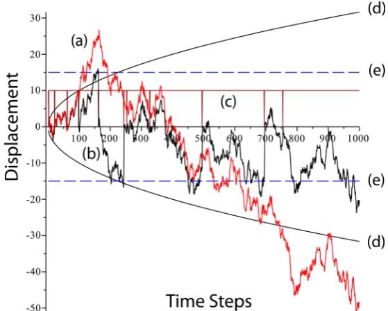
1, 0 of a binomial random generator, scaled by a factor 5 for better visibility in the plot. A sample of 500 Bernoulli trials with probability of decay of 1% is expected to yield 5 2± de-cays. In the illustrated run, 4 decays occurred where the brown trace plunges sharply from 5 to 0. The solid black trace is the Brownian trajectory of the de-caying particle. At each occurrence of decay, the trajectory plunges to 0 and the process is terminated. A new process then begins as represented by the portion of the red trace recommencing at the origin and continuing until the next decay, whereupon the process of termination and commencement repeats. Whereas the TPF is a continuous conditional probability function that shows how the distri-bution of displacements of a single particle evolves in time, provided the particle has not decayed, the numerical solutions to the stochastic differential equation permit one to see in real time the discontinuous nature of diffusion with decay. The horizontal dashed blue lines in the figure represent boundaries that will be discussed briefly in connection with Figure 2 and in greater detail in Section 3.

(16)

[image:16.595.238.511.69.300.2]

Figure 1. Computer simulation of Brownian motion with decay. Parameters: n=500

time steps dt=1 with diffusivity D=0.5 and survival probability ps=0.99. (a)

Dis-placement of stable particle (solid red). (b) DisDis-placement of unstable particle (solid black); each decay event terminates the process, which recommences with a new particle. (c) Se-quence of Bernoulli trials (solid brown) each with possible outcomes ε =

( )

1, 0 scaled up by factor of 5 for clarity; outcome ε =0 signifies particle decay. (d) Parabolic branches (light black) of the root-mean-square displacement σ

( )

t = 2Dt. (e)

Absorb-ing boundaries (dashed blue) at xb= ±15.

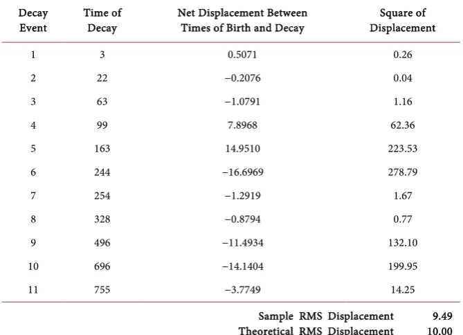
Figure 2. Computer simulation of Brownian motion with decay, employing n=1000

[image:16.595.233.513.429.653.2]

(17)

Moreover, there is no formal “law of averages”; the closest rigorous principle would be the law of large numbers [Ref [33], pp. 190-191]. What a correctly formulated law of large numbers does imply is that over many repetitions of a random walk starting from the same initial conditions the ensemble of Brownian trajectories will be found in the positive half-space to approximately the same extent as in the negative half-space [Ref [18], p. 372]. The simulated Brownian trajectories (black) of the unstable particle in Figure 1 is consistent with this im-plication. Upon several repetitions of the random walk by a new particle after decay of a previous one, the ensemble of resulting trajectories, obtained by downward projection of the red trace, shows a more equal balance of time be-tween the two half spaces.

Figure 2 shows a simulation of longer duration n=1000 for the same values

of D and ps as in Figure 1. In this simulation the trajectory (red) of the stable

particle starts out at the origin, moves again into the positive half-space, but crosses the origin at around 400 and then spends approximately 61% of the total duration, in the negative half-space. A decay probability of 1% is expected to yield 10 3± decays in 1000 Bernoulli trials; the simulation in Figure 2 yielded

11 events, as shown by the horizontal brown trace (scaled by a factor 10 for clar-ity) with sharp drops to 0 at each decay. The corresponding partition of the con-tinuous trajectory into the disjointed trajectories of 11 sequentially decaying particles is still unequally distributed over the two half-spaces because 1000 time steps is too short a duration, and 11 decays lead to too small an ensemble of tra-jectories. Simulations of n=5000 or more, not reproduced here, show closer

conformity to the law of large numbers.

The black trajectories of Figure 2 permit confirmation of a significant feature of the Brownian motion of an unstable particle that is addressed in Section 3, viz.

the question of exit time, i.e. how much time, on average, is required for the par-ticle to reach one of the two absorbing boundaries arbitrarily set at = ±15 as

marked by dashed blue lines. Since the characteristics of Brownian motion are independent of where or when the motion begins, a new Brownian trajectory starts at the origin following each particle decay, and the random walk of the particle to either boundary terminates the process. In Section 3 the expectation of the exit time is (a) derived for a decaying particle, (b) compared with the em-pirical result deduced from Figure 2, and (c) shown to differ markedly from the theoretical result for a stable particle.

2.4. Langevin Equation: Analytical Solution

(18)

Consider first the misleading (or at least incomplete) way to proceed. If one regards the numerical update algorithm (41) as a sum of n independent unit normal variates multiplied by Bernoulli variates all taken to have value

ε

=1,

then X t

( )

must also be expressible in closed form as a normal random

varia-ble of zero mean because of the stability of the normal distribution. Moreover, since a normal distribution is uniquely determined by the mean and variance, it follows from relation (44) that the solution (in the limit n td →t) must be

( )

2

(

)

0, D 1 e t

X t N λ

λ −

 

= _ − _

 , (58)

whereupon the corresponding PDF, generalized on the basis of space and time translational symmetry to include initial conditions

(

x t0,0

)

, takes the form

( )

(

)

( )

(

0

)

(

)

(

( 0)

)

2 L

0 0 0

1

, , exp 4 1 e

4π 1 e

t t X

t t

p x t x t x x D D

λ

λ _λ λ

− − − −

= − − −

− .(59)

The superscript L distinguishes solution (59) to the Langevin stochastic equa-tion from soluequa-tion (20) to the Fokker-Planck equaequa-tion repeated below for ease of comparison

( )

(

)

(

)

(

)

(

)

( 0)

2 FP

0 0 0 0

0

1

, , exp 4 e

4π

t t X

p x t x t x x D t t

D t t

λ − −

= − − −

− (60)

and denoted by a superscript FP.

The problem with solution (58), however, is that it no longer describes a process that can be interrupted at any time by the decay of the particle. The transformation from a discontinuous to a continuous stochastic process arose by confounding the Bernoulli random variables, which can be either 1 or 0, with the specific outcomes, or variates, all taken to be 1 in the previous calculation of ex-pectation values. Re-examining the last line in Equation (41)—i.e. before expec-tation values are taken—shows, together with the stability of the normal distri-bution, that Langevin Equation (40), expressed in terms of random variables, can be written as

( )

_d

( )

(

_{0, 2 d} 2

)

n

X n t ≡X t =N D tΣ

(61) in which

2 2 2 2 2

1 2 3

n n n

n j j j n

j j j

ε ε ε ε

= = =

Σ =

∏

+

∏

+

∏

+ +_

(62) is a random variable, not an expectation value. So as not to complicate the nota-tion unnecessarily, the symbol for a Bernoulli random variable will remain ε_, in departure from the conventional notation to use an upper-case letter.

The question then becomes: What kind of random variable is 2 n

Σ _{and what}

are its properties? Details of the analysis are left to Appendix 1, but the salient points are summarized as follows. Any random variable Z is uniquely characte-rized by its moment-generating function (MGF)

( )

exp

( )

Z

g θ ≡ Zθ

(19)

(if it exists), or its characteristic function (CF)

( )

exp

(

)

Z

h θ ≡ iZθ

(64) (which always exists), or its probability function (for discrete outcomes) or probability density (for continuous outcomes) [34]. The variable

θ

in the ar-gument of relations (63) and (64) has no physical significance, but merely serves as a dummy variable for purposes of differentiation, after which it is set equal to 0. In the analysis of 2

n

Σ _{in Appendix 1, the MGF was used progressively,}

start-ing from the relation ε=B

(

1,p_s

)

, to show that

(

) (

)

2

1, 1, 2, ,

j j B ps j n

ε

=

ε

= = _

(65)

(

)

(

)

2 1

1, 1, 2, ,

n n

n j

j k k s

k j k j

B p j n

ω ε ε − +

= = ≡

∏

=

∏

= = 

(66) and 2 1 n n j j ω =

Σ ≡

∑

_{. (67)}

If the set of random variables

{ }

ωj were mutually independent, the MGF of

the sum in (67) could be easily calculated. However, by virtue of the defining re-lation (66), any pair of the ω _{variables, e.g.}

ω

_j=

ε ε

_j _j+₁

ε ε

_k _k+₁

ε

_n and

1

k k k n

ω =ε ε +ε , could contain some identical factors and be highly correlated. Nevertheless, although less easily done, the MGF of 2

n

Σ _{can be shown to be}

( )

(

)

(

)

2

1

1 e 1 e

1 e n n n s s s p p g p θ θ θ

θ

+ Σ − + − =

− . (68) Although MGF (68) does not correspond to any of the tabulated random va-riables known to the author, all the moments of 2

n

Σ _{can be determined by}

dif-ferentiation

( )

2

( )

( ) (

)

2 2

0 d

0 0,1, 2,

d k k _k n k g g k θ θ θ Σ Σ =

Σ = ≡ = _ _,

₍₆₉₎

thereby characterizing 2 n

Σ uniquely.

For example, moments k=0,1, 2 of Σ2n calculated from (68) and (69) are

( )

(

)

( )

(

)

(

)

(

)

2 2 2 0 ₀ 2 1 ₁ 2 1 2 ₂ 2 2 0 1 1 0 1

1 1 ₂

0 1 1 n n s s n s n _n

s s s _s

n s s g p p g p

p p p _np g p p Σ Σ + Σ

Σ = =

−

Σ = =

−

+ −

Σ = = −

−

(70)

(20)

( )

(

)

2

(

₂

)

2 ₂

(

1

)

0, 2 d 2 d 2 d

1 n s s n n s p p X t N D t D t D t

p

 − 

 

= Σ = Σ =

 − 

 

, (71)

leads to

( )

(

)

2

(

)

(

)

(

)

d 0

1 d 1 1 d ₂

lim 2 d 1 e

d

n

t n

t

t t _D

X t D t

t λ λ λ λ λ − →∞ →   ₋ _{− −}     = _ _ __= −    _ _   (72)

upon substitution of relation (27) for ps and transforming from discrete time

steps to continuous time. The expectation value (72) is precisely the result ob-tained by a different procedure in (44) and justifies the form of PDF (59). The third line of (70) enables one to calculate the variance of 2

n

Σ and the 4th

mo-ment of the displacemo-ment

( )

(

)

4 2

( )

2

( )

2 2 2

(

)

2 d 0

8

lim 4 d n 1 1 e t

n t

D

X t D t λt λ

λ

− →∞

→

 

= _ Σ _= − +

 

(73)

by means of the same substitution and limiting process employed in Equation (72).

In short, therefore, the solution (61) takes the form of a normal distribution whose variance is itself a random variable of un-named variety (as far as the au-thor is aware), but which is completely and uniquely specified by its MGF (68). In principle, the PDF of the distribution of 2

n

Σ _{can be calculated by taking the}

inverse Fourier transform of the CF; the CF itself is obtained simply by substi-tuting i

θ

for

θ

in the MGF (68). For the purposes of this paper, however, the

PDF of 2 n

Σ _{is not required.}

Solution (61), in contrast to solution (58), incorporates the Bernoulli processes that generate particle decay. If, in a simulation of Brownian motion to be implemented for n time steps from Equation (61), the Bernoulli variate

0

k

ε = _{at time step}k≤n, it follows from Equation (66) that all the variates 0

j

ω

= _for j=1, 2,,k, and therefore Σ =2_k 0, and X t

(

=k td

)

=N

( )

0, 0 =0. (Note: N

( )

0, 0 =0 signifies that

(

1

(

2 2

)

0

lim exp x 2 0

σ

−

→ − = of the Gaussian

PDF.) Thus, the random walk of the decayed particle has been realistically ter-minated at the randomly selected th

k time step. With regard to notation, the

subscript on 2 n

Σ _{can be taken to represent the full length (}_i.e._{number of time}

steps) of a simulated random walk, and not (as before) a pre-determined num-ber of sequential steps survived by the particle. In the limit of an infinitely long random walk, it follows from Equation (72) that the (infinitely) many particle trajectories arising from the introduction of a new particle after decay of each previous one, yield a root-mean-square (RMS) displacement equal to the ma-thematical diffusion length 2D

λ

, in accord with the ensemble averages (53)

and (57).

(21)

[image:21.595.206.541.103.345.2]

Table 1. Test of Theoretical Ensemble-Averaged RMS Displacement Using Simulated

Trajectories of Figure 2.

Decay

Event Time of Decay Net Displacement Between Times of Birth and Decay Displacement Square of

1 3 0.5071 0.26

2 22 −0.2076 0.04

3 63 −1.0791 1.16

4 99 7.8968 62.36

5 163 14.9510 223.53

6 244 −16.6969 278.79

7 254 −1.2919 1.67

8 328 −0.8794 0.77

9 496 −11.4934 132.10

10 696 −14.1404 199.95

11 755 −3.7749 14.25

Sample RMS Displacement 9.49 Theoretical RMS Displacement 10.00

chronologically the decay events and corresponding times of decay. Columns 3 and 4 show the net displacement (to 4 significant figures) and square of dis-placement (truncated to 2 significant figures) between the time of creation of the particle at the origin x0=0 up to the time step just prior to its decay. As shown, the mean of the 11 RMS values is very close to the theoretical prediction calculated from Equation (53) with the parameters used in the simulations of

Figure 2: D=0.5, dt=1, ps=0.99, in which case λ= −

(

1 ps

)

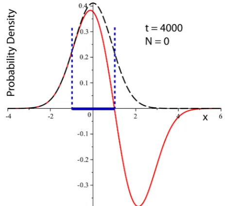
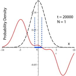
dt=0.01.

Now that the stochastically correct solution (61) to the Langevin equation has been derived and shown to justify PDF (59), it is informative to compare the lat-ter with PDF (60) derived from the Fokker-Planck Equation (18). Figure 3 and

Figure 4 respectively show plots of the Langevin and Fokker-Planck PDFs as a

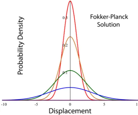
function of displacement for different random walk durations. The principal feature to notice is that, as the duration of the random walk increases, the PDF derived from the Langevin solution approaches a steady-state Gaussian distribu-tion of mean 0, maximum

(

)

1 2

4πDλ − , and variance 2Dλ, whereas the

dis-tribution derived from the Fokker-Planck solution vanishes, i.e. approaches a Gaussian distribution of mean 0, maximum 0, and infinite width. In light of the previous discussion, these differences are understandable as follows:

• _{The Fokker-Planck Equation (18), although it includes the particle decay rate,}

describes one long continuous process, i.e. the evolution of the probability of a particular diffusing particle to be found at an arbitrary location x at time t, provided the particle survived to time t. As t increases, the survival probabil-ity of that particular particle decreases exponentially as e−λt, and the mean-

(22)

However, only after an infinitely long time is the probability for the particle to reach any location precisely zero.

• _{In contrast to the preceding, the Langevin Equation (40) describes a}

poten-tially infinite number of independent Brownian trajectories, disconnected one from the other by events of particle decay. As t increases, the ensemble of independent trajectories come from particles that have survived for different lengths of time. In the limit of an infinitely long time, the probability density (59) does not vanish, but describes, instead, the ensemble-averaged statistics characterized by a Gaussian distribution with mean-square displacement

[image:22.595.259.487.232.423.2]

2Dλ.

Figure 3. Spatial variation of the probability density function (59) obtained from solution

of the Langevin stochastic Equation (40) for time units t = 1 (red), 2 (gold), 5 (green), 10 (blue), infinite (violet). Process parameters are initial location x0=0, diffusivity

0.5

D= , decay rate λ =0.1.

Figure 4. Spatial variation of the probability density function (60) obtained from solution

[image:22.595.258.484.491.680.2]

(23)

[image:23.595.251.496.64.264.2]

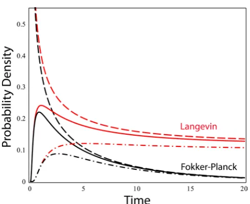
Figure 5. Temporal variation of the probability density function (59) of the Langevin

Equation (red) and (60) of the Fokker-Planck Equation (black) for spatial coordinates x = 0 (dash), 1 (solid), 2 (dot-dash). Process parameters are diffusivity D=0.5, decay rate

0.1

λ = _.

Further perspective on the differences between the two approaches (Langevin vs Fokker-Planck) is given by Figure 5, which shows plots of PDFs (59) and (60) as a function of time for several different locations. The probability for a particle to remain at the origin

(

x0=0

)

decreases monotonically in both cases, but asymptotically approaches 0 in the Fokker-Planck PDF and

(

)

1 2

4πDλ − in the

Langevin PDF. The probability for a particle to remain at a location away from the origin is 0 to begin with, due to the imposed boundary condition (19) which applies to both PDFs, rises to a maximum, and subsequently decreases to the preceding asymptotic limits.

It is to be emphasized that the Fokker-Planck and Langevin descriptions are both valid. It is not that one is right and the other wrong; rather, the two analyt-ical methods provide different perspectives on the process of Brownian motion with decay. The Fokker-Planck equation describes a continuous process; it gives a statistical description of the displacement of a decaying particle for as long as the particle might survive in the course of an infinite time span. The Langevin equation describes a sequence of discontinuous processes; it gives a statistical description of the displacement of an ensemble of particles up to the instant each actually fails to survive. It is understandable, therefore, why the theoretical mean-square displacements obtained by the two approaches are different. A sig-nificant point of this paper, however, is that for stable particles the two ap-proaches lead to identical results because both would then be describing a single continuous process of infinite duration.

3. First-Passage Times

(24)

other unstable particles undergoing Brownian motion: At what time will the particle, starting from a given point (e.g. x0=0), first reach some other speci-fied location? This is the problem of first-passage time (FPT) or exit time. If, upon reaching the designated location, the particle is removed from the system, the location is said to be an absorbing boundary. At an absorbing boundary, the probability density vanishes. Other kinds of boundaries can be transmitting, i.e.

have no effect on the particle’s subsequent motion, or reflecting, in which case the particle current density, but not probability density, vanishes. This paper is concerned with absorbing boundaries, since these conditions characterize a va-riety of measurement protocols employing passive diffusion of radioactive atoms in gas, aerosol, and dust, as well as unstable molecules in a fluid medium..

In Figure 1 and Figure 2, two absorbing boundaries were arbitrarily set at

15

b

x = ± units from the origin. As shown in Figure 1, the unstable particle

(black) first reached boundary xb= +15 at approximately tb=125 before

de-caying at td2=250. Note, however, that a prior decay occurred close to 1 33

d

t = . Therefore the first particle did not reach the boundary before decaying,

and the second particle, which began a new process, reached the boundary after a diffusion time of tb−td1=92. In the simulation shown in Figure 2, there are four decays, the last occurring at time step td4=99, before the fifth unstable particle reached boundary xb= +15 for the first time at time step tb=158, and

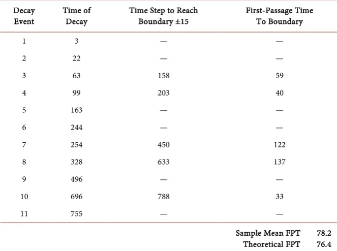
then decayed shortly afterward at time step td5=163. The FPT for particle 5 is therefore tb−td4=59. In a FPT problem with unstable particles and absorbing boundaries, the process of Brownian motion is terminated by decay or by reach-ing a boundary; there is no second-passage time. Table 2, which will be used shortly to test an important theoretical result, summarizes all the first-passage times of the trajectories in Figure 2.

FPT problems have been studied in great detail for non-decaying diffusers; see, for example [23]. In this paper, however, the problem of FPT is solved for unsta-ble diffusers. Since the FPT is a random variaunsta-ble, for which the symbol T will again be used, solving the FPT problem ordinarily means calculating the expec-tation value TFPT