113
Evaluating Recurrent Neural Network Explanations
Leila Arras1, Ahmed Osman1, Klaus-Robert M ¨uller2,3,4, and Wojciech Samek1
1Machine Learning Group, Fraunhofer Heinrich Hertz Institute, Berlin, Germany 2Machine Learning Group, Technische Universit¨at Berlin, Berlin, Germany 3Department of Brain and Cognitive Engineering, Korea University, Seoul, Korea
4Max Planck Institute for Informatics, Saarbr¨ucken, Germany {leila.arras, wojciech.samek}@hhi.fraunhofer.de
Abstract
Recently, several methods have been proposed to explain the predictions of recurrent neu-ral networks (RNNs), in particular of LSTMs. The goal of these methods is to understand the network’s decisions by assigning to each in-put variable, e.g., a word, arelevance indicat-ing to which extent it contributed to a partic-ular prediction. In previous works, some of these methods were not yet compared to one another, or were evaluated only qualitatively. We close this gap by systematically and quan-titatively comparing these methods in differ-ent settings, namely (1) a toy arithmetic task which we use as a sanity check, (2) a five-class sentiment prediction of movie reviews, and be-sides (3) we explore the usefulness of word relevances to build sentence-level representa-tions. Lastly, using the method that performed best in our experiments, we show how specific linguistic phenomena such as the negation in sentiment analysis reflect in terms of relevance patterns, and how the relevance visualization can help to understand the misclassification of individual samples.
1 Introduction
Recurrent neural networks such as LSTMs (Hochreiter and Schmidhuber, 1997) are a stan-dard building block for understanding and gener-ating text data in NLP. They find usage in pure NLP applications, such as abstractive summa-rization (Chopra et al., 2016), machine transla-tion (Bahdanau et al., 2015), textual entailment (Rockt¨aschel et al., 2016); as well as in multi-modal tasks involving NLP, such as image cap-tioning (Karpathy and Fei-Fei,2015), visual ques-tion answering (Xu and Saenko,2016) or lip read-ing (Chung et al.,2017).
As these models become more and more widespread due to their predictive performance, there is also a need to understand why they took
a particular decision, i.e., when the input is a se-quence of words: which words are determinant for the final decision? This information is crucial to unmask “Clever Hans” predictors (Lapuschkin et al.,2019), and to allow for transparency of the decision-making process (EU-GDPR,2016).
Early works onexplainingneural network pre-dictions includeBaehrens et al.(2010);Zeiler and Fergus(2014);Simonyan et al.(2014); Springen-berg et al. (2015); Bach et al. (2015); Alain and Bengio(2017), with several works focusing on ex-plaining the decisions of convolutional neural net-works (CNNs) for image recognition. More re-cently, this topic found a growing interest within NLP, amongst others to explain the decisions of general CNN classifiers (Arras et al., 2017a; Ja-covi et al.,2018), and more particularly to explain the predictions of recurrent neural networks (Li et al.,2016,2017;Arras et al.,2017b;Ding et al.,
2017;Murdoch et al.,2018;Poerner et al.,2018). In this work, we focus on RNN explanation methods that are solely based on a trained neu-ral network model and a single test data point1. Thus, methods that use additional information, such as training data statistics, sampling, or are optimization-based (Ribeiro et al., 2016; Lund-berg and Lee, 2017; Chen et al., 2018) are out of our scope. Among the methods we consider, we note that the method ofMurdoch et al.(2018) was not yet compared againstArras et al.(2017b);
Ding et al. (2017); and that the method of Ding et al. (2017) was validated only visually. More-over, to the best of our knowledge, no recurrent neural network explanation method was tested so far on a toy problem where theground truth
rele-1
vance value is known.
Therefore our contributions are the follow-ing: we evaluate and compare the aforementioned methods, using two different experimental setups, thereby we assess basic properties and differences between the explanation methods. Along-the-way we purposely adapted a simple toy task, to serve as a testbed for recurrent neural networks explana-tions. Lastly, we explore how word relevances can be used to build sentence-level representations, and demonstrate how the relevance visualization can help to understand the (mis-)classification of selected samples w.r.t. semantic composition.
2 Explaining Recurrent Neural Network Predictions
First, let us settle some notations. We suppose given a trained recurrent neural network based model, which has learned some scalar-valued pre-diction functionfc(·), for each classc of a clas-sification problem. Further, we denote by x = (x1,x2, ...,xT)an unseen input data point, where
xtrepresents thet-th input vector of dimensionD, within the input sequencexof lengthT. In NLP, the vectorsxtare typically word embeddings, and xmay be a sentence.
Now, we are interested in methods that can ex-plain the network’s prediction fc(x) for the in-putx, and for a chosentarget classc, by assign-ing a scalar relevance value to each input variable or word. This relevance is meant to quantify the variable’s or word’s importance for or against a model’s predictiontowardsthe classc. We denote by Rxi (index i) the relevance of a single
vari-able. This means xi stands for any arbitrary in-put variablext,d representing thed-th dimension, d∈ {1, ..., D}, of an input vectorxt. Further, we refer toRxt (index t) to designate the relevance
value of anentireinput vector or word xt. Note that, for most methods, one can obtain a word-level relevance value by simply summing up the relevances over the word embedding dimensions, i.e.Rxt =
P
d∈{1,...,D}Rxt,d.
2.1 Gradient-based explanation
One standard approach to obtain relevances is based on partial derivatives of the prediction func-tion: Rxi =
∂f∂xc
i(x)
, orRxi = ∂f∂xc
i(x)
2
( Di-mopoulos et al., 1995; Gevrey et al., 2003; Si-monyan et al.,2014;Li et al.,2016).
In NLP this technique was employed to
visual-ize the relevance of single input variables in RNNs for sentiment classification (Li et al., 2016). We use the latter formulation of relevance and denote it asGradient. With this definition the relevance of an entire word is simply the squaredL2-norm
of the prediction function’s gradient w.r.t. the word embedding, i.e.Rxt =k∇xt fc(x)k
2 2.
A slight variation of this approach uses partial derivatives multiplied by the variable’s value, i.e.
Rxi =
∂fc
∂xi(x)·xi. Hence, the word relevance is a
dot product between prediction function gradient and word embedding: Rxt = (∇xt fc(x))
Tx t (Denil et al., 2015). We refer to this variant as
Gradient×Input.
Both variants are general and can be applied to any neural network. They are computationally ef-ficient and require one forward and backward pass through the net.
2.2 Occlusion-based explanation
Another method to assign relevances to single variables, or entire words, is by occluding them in the input, and tracking the difference in the net-work’s prediction w.r.t. a prediction on the orig-inal unmodified input (Zeiler and Fergus, 2014;
Li et al.,2017). In computer vision the occlusion is performed by replacing an image region with a grey or zero-valued square (Zeiler and Fergus,
2014). In NLP word vectors, or single of its com-ponents, are replaced by zero; in the case of re-current neural networks, the technique was applied to identify important words for sentiment analysis (Li et al.,2017).
Practically, the relevance can be computed in two ways: in terms of prediction function dif-ferences, or in the case of a classification prob-lem, using a difference of probabilities, i.e.Rxi =
fc(x)−fc(x|xi=0), orRxi =Pc(x)−Pc(x|xi=0),
where Pc(·) = Pexpfc(·)
kexpfk(·). We refer to the
former as Occlusionf-diff, and to the latter as OcclusionP-diff. Both variants can also be used to
estimate the relevance of an entire word, in this case the corresponding word embedding is set to zero in the input. This type of explanation is computationally expensive and requiresTforward passes through the network to determine one rele-vance value per word in the input sequencex.
omis-sion was shown to deliver inferior results, there-fore we consider only occlusion-based relevance.
2.3 Layer-wise relevance propagation
A general method to determine input space rele-vances based on a backward decomposition of the neural network prediction function is layer-wise relevance propagation (LRP) (Bach et al., 2015). It was originally proposed to explain feed-forward neural networks such as convolutional neural net-works (Bach et al.,2015;Lapuschkin et al.,2016), and was recently extended to recurrent neural net-works (Arras et al., 2017b; Ding et al., 2017;
Arjona-Medina et al.,2018).
LRP consists in a standard forward pass, fol-lowed by a specific backward pass which is de-fined for each type of layer of a neural network by dedicated propagation rules. Via this backward pass, each neuron in the network gets assigned a relevance, starting with the output neuron whose relevance is set to the prediction function’s value, i.e. to fc(x). Each LRP propagation rule redis-tributes iteratively, layer-by-layer, the relevance from higher-layer neurons to lower-layer neurons, and verifies a relevance conservation property2. These rules were initially proposed inBach et al.
(2015) and were subsequently justified by Deep Taylor decomposition (Montavon et al.,2017) for deep ReLU nets.
In practice, for a linear layer of the formzj =
P
iziwij+bj , and given the relevances of the out-put neuronsRj, the input neurons’ relevancesRi are computed through the following summation:
Ri =Pj
zi·wij
zj+·sign(zj) ·Rj, whereis a stabilizer
(small positive number); this rule is commonly re-ferred as-LRP or-rule3. With this redistribution the relevance is conserved, up to the relevance as-signed to the bias and “absorbed” by the stabilizer. Further, for an element-wise nonlinear activa-tion layer, the output neurons’ relevances are re-distributed identically onto the input neurons.
In addition to the above rules, in the case of a multiplicative layer of the form zj = zg ·zs,
Arras et al. (2017b) proposed to redistribute zero relevance to the gate (the neuron that is sigmoid
2Methods based on a similar conservation principle
in-clude contribution propagation (Landecker et al., 2013), Deep Taylor decomposition (Montavon et al., 2017), and DeepLIFT (Shrikumar et al.,2017).
3Such a rule was employed by previous works with
recur-rent neural networks (Arras et al.,2017b;Ding et al.,2017; Arjona-Medina et al.,2018), although there exist also other LRP rules for linear layers (see e.g.Montavon et al.,2018)
activated) i.e. Rg = 0, and assign all the rele-vance to the remaining signal neuron (which is usually tanh activated) i.e.Rs =Rj. We call this LRP variant LRP-all, which stands for “signal-take-all” redistribution. An alternative rule was proposed in Ding et al. (2017); Arjona-Medina et al.(2018), where the output neuron’s relevance
Rj is redistributed onto the input neurons via: Rg = zgz+gzsRj and Rs = zgz+szsRj. We re-fer to this variant asLRP-prop, for “proportional” redistribution. We also consider two other vari-ants. The first one uses absolute values instead:
Rg =
|zg|
|zg|+|zs|Rj and Rs =
|zs|
|zg|+|zs|Rj, we
call it LRP-abs. The second uses equal redistri-bution: Rg = Rs = 0.5 ·Rj (Arjona-Medina
et al.,2018), we denote it asLRP-half. We further add a stabilizing term to the denominator of the
LRP-propandLRP-absformulas, it has the form
·sign(zg +zs)in the first case, and simplyin the latter.
Since the relevance can be computed in one for-ward and backfor-ward pass, the LRP method is ef-ficient. Besides, it is general as it can be ap-plied to any neural network made of the above lay-ers: it was applied successfully to CNNs, LSTMs, GRUs, and QRNNs (Poerner et al., 2018; Yang et al.,2018)4.
2.4 Contextual Decomposition
Another method, specific to LSTMs, is contextual decomposition (CD) (Murdoch et al., 2018). It is based on alinearizationof the activation func-tions that enables to decompose the LSTM for-ward pass by distinguishing between two contri-butions: those made by a chosen contiguous sub-sequence (a word or a phrase) within the input se-quence x, and those made by the remaining part of the input. This decomposition results in a fi-nal hidden state vector hT (see the Appendix for a full specification of the LSTM architecture) that can be rewritten as a sum of two vectors: βT and γT, where the former corresponds to the contribu-tion from the “relevant” part of interest, and the latter stems from the “irrelevant” part. When the LSTM is followed by a linear output layer of the formwTchT +bc for classc, then the relevance of a given word (or phrase) and for thetargetclassc, is given by the dot product:wTcβT.
4Note that in the present work we apply LRP to
Method Relevance Formulation Redistributed Quantity (P
iRxi) Complexity
Gradient Rxi =
∂fc ∂xi(x)
2
k∇xfc(x)k22 Θ(2·T)
Gradient×Input Rxi =
∂fc
∂xi(x)·xi (∇xfc(x))
Tx Θ(2·T)
Occlusion Rxi =fc(x)−fc(x|xi=0) - Θ(T
2)
LRP backward decomposition of the neurons’ relevance fc(x) Θ(2·T)
CD linearization of the activation functions fc(x) Θ(T2)
Table 1: Overview of the considered explanation methods. The last column indicates the computational complexity to obtain one relevance value per input vector, or word, whereT is the length of the input sequence.
The method is computationally expensive as it requires T forward passes through the LSTM to compute one relevance value per word. Although it was recently extended to CNNs (Singh et al.,
2019;Godin et al.,2018), it is yet not clear how to compute theCDrelevance in other recurrent archi-tectures, or in networks with multi-modal inputs.
See Table 1for an overview of the explanation methods considered in the present work.
2.5 Methods not considered
Other methods to compute relevances include In-tegrated Gradients (Sundararajan et al.,2017). It was previously compared againstCDinMurdoch et al. (2018), and against the LRP variant of Ar-ras et al.(2017b) inPoerner et al.(2018), where in both cases it was shown to deliver inferior results. Another method is DeepLIFT ( Shriku-mar et al., 2017), however, according to its au-thors, DeepLIFT was not designed for multiplica-tive connections, and its extension to recurrent net-works remains an open question5. For a compar-ative study of explanation methods with a main focus on feed-forward nets, see Ancona et al.
(2018)6. For a broad evaluation of explanations, including several recurrent architectures, we refer toPoerner et al.(2018). Note that the latter didn’t include theCDmethod ofMurdoch et al.(2018), and the LRP variant ofDing et al.(2017), which we compare here.
5
ThoughPoerner et al.(2018) showed that, when using only the Rescale rule of DeepLIFT, and combining it with the product rule proposed inArras et al.(2017b), then the resulting explanations perform on-par with the LRP method ofArras et al.(2017b)
6
Note that in order to redistribute the relevance through product layers,Ancona et al.(2018) simply relied on standard gradient backpropagation. Such a redistribution scheme is not appropriate for methods such as LRP, since it violates the relevance conservation property, hence their results for recurrent nets are not conclusive.
3 Evaluating Explanations
3.1 Previous work
How to generally and objectively evaluate expla-nations, without resorting to ad-hoc evaluation procedures that are domain and task specific, is still active research (Alishahi et al., 2019; Be-linkov and Glass,2019).
In computer vision, it has become common practice to conduct a perturbation analysis (Bach et al.,2015;Samek et al.,2017;Shrikumar et al.,
2017; Lundberg and Lee, 2017; Ancona et al.,
2018; Chen et al., 2018; Morcos et al., 2018): hereby a few pixels in an image are perturbated (e.g. set to zero or blurred) according to their rel-evance (most relevant or least relevant pixels are perturbated first), and then the impact on the net-work’s prediction is measured. The higher the im-pact, the more accurate is the relevance.
Other studies explored in which way relevances are consistent or helpful w.r.t. human judgment (Ribeiro et al., 2016; Lundberg and Lee, 2017;
Nguyen, 2018). Some other works relied solely on the visual inspection of a few selected rel-evance heatmaps (Li et al., 2016; Sundararajan et al.,2017;Ding et al.,2017).
In NLP, Murdoch et al. (2018) proposed to measure the correlation between word relevances obtained on an LSTM, and the word impor-tance scores obtained from a linear Bag-of-Words. However, the latter model ignores the word order-ing and context, which the LSTM can take into account, hence this type of evaluation is not ad-equate7. Other evaluations in NLP are task spe-cific. For example Poerner et al. (2018) use the subject-verb agreement task proposed by Linzen et al.(2016), where the goal is to predict a verb’s
7
number, and use the relevances to verify that the most relevant word is indeed the correct subject (or a noun with the predicted number).
Other studies include an evaluation on a syn-thetic task: Yang et al.(2018) generated random sequences of MNIST digits and train an LSTM to predict if a sequence contains zero digits or not, and verify that the explanation indeed assigns a high relevance to the zero digits’ positions.
A further approach uses randomization of the model weights and data as sanity checks (Adebayo et al.,2018) to verify that the explanations are in-deed dependent on the model and data. Lastly, some evaluations are “indirect” and use relevances to solve a broader task, e.g. to build document-level representations (Arras et al., 2017a), or to redistribute predicted rewards in reinforcement learning (Arjona-Medina et al.,2018).
3.2 Toy Arithmetic Task
As a first evaluation, we ask the following ques-tion: if we add two numbers within an input se-quence, can we recover from the relevance the true input values? This amounts to consider the adding problem (Hochreiter and Schmidhuber,
1996), which is typically used to test the long-range capabilities of recurrent models (Martens and Sutskever, 2011; Le et al., 2015). We use it here to test the faithfulness of explanations. To that end, we define a setup similar to Hochre-iter and Schmidhuber(1996), but withoutexplicit
markers to identify the sequence start and end, and the two numbers to be added. Our idea is that, in general, it is not clear what the ground truth rele-vance for a marker should be, and we want only the relevant numbers in the input sequence to get a non-zero relevance. Hence, we represent the input sequencex = (x1,x2, ...,xT) of lengthT, with two-dimensional input vectors as:
( 0 0 0 na 0 0 0 nb 0 0 0
n1 ... na−1 0 na+1... nb−1 0 nb+1... nT)
where the non-zero entries nt are random real numbers, and the two relevant positionsaandbare sampled uniformly among{1, ..., T}witha < b.
More specifically, we consider two tasks that can be solved by an LSTM model with a hidden layer of sizeone(followed by a linear output layer with no bias8): theadditionof signed numbers (nt
8We omit the output layer bias since all considered
expla-nation methods ignore it in the relevance computation, and we want to explain the “full” prediction function’s value.
is sampled uniformly from[−1,−0.5]∪[0.5,1.0]) and thesubtractionof positive numbers (ntis sam-pled uniformly from [0.5,1.0]9). In the former case the target output y is na +nb, in the latter it isna−nb. During training we minimize Mean Squared Error (MSE). To ensure that train/val/test sets do not overlap we use 10000 sequences with lengths T ∈ {4, ...,10} for training, 2500 se-quences with T ∈ {11,12} for validation, and 2500 sequences with T ∈ {13,14} as test set. For each task we train 50 LSTMs with a validation MSE<10−4, the resulting test MSE is<10−4.
Then, given the model’s predicted outputypred,
we compute one relevance value Rxt per input
vectorxt (for the occlusion method we compute onlyOcclusionf-diffsince the task is a regression;
we also don’t reportGradientresults since it per-forms poorly). Finally, we track the correlation between the relevances and the two input numbers
naandnb. We also track the portion of relevance assigned to the relevant time steps, compared to the relevance for all time steps. Lastly, we cal-culate the “MSE” between the relevances for the relevant positionsaandband the model’s output. Our results are compiled in Table2.
Interestingly, we note that on the addition task several methods perform well and produce a rele-vance that correlates perfectly with the input num-bers: Gradient×Input, Occlusion, LRP-all and
CD (they are highlighted in bold in the Table). They further assign all the relevance to the time stepsaandband almost no relevance to the rest of the input; and present a relevance that sum up to the predicted output. However, on subtraction, onlyGradient×InputandLRP-allpresent a corre-lation of near one withna, and of near minus one withnb. Likewise these methods assign only rele-vance to the relevant positions, and redistribute the predicted output entirely onto these positions.
The main difference between our addition and subtraction tasks, is that the former requires only summing up the first dimension of the input vec-tors and can be solved by a Bag-of-Words ap-proach (i.e. by ignoring the ordering of the in-puts), while our subtraction task is truly sequen-tial and requires the LSTM model to remember which number arrived first, and which number ar-rived second, via exploiting the gating mechanism. Since in NLP several applications require the
9We avoid small numbers by using 0.5 as a minimum
ρ(Rxa, na) ρ(Rxb, nb) E[
|Rxa|+|Rxb|
P
t|Rxt| ] E[((Rxa+Rxb)−ypred)2]
(in %) (in %) (in %) (“MSE”)
Toy Task Addition
Gradient×Input 99.960(0.017) 99.954(0.019) 99.68(0.53) 24.10−4(8.10−4) Occlusion 99.990(0.004) 99.990(0.004) 99.82(0.27) 20.10−5(8.10−5)
LRP-prop 0.785 (3.619) 10.111 (12.362) 18.14 (4.23) 1.3 (1.0) LRP-abs 7.002 (6.224) 12.410 (17.440) 18.01 (4.48) 1.3 (1.0) LRP-half 29.035 (9.478) 51.460 (19.939) 54.09 (17.53) 1.1 (0.3) LRP-all 99.995(0.002) 99.995(0.002) 99.95(0.05) 2.10−6(4.10−6) CD 99.997(0.002) 99.997(0.002) 99.92(0.06) 4.10−5(12.10−5)
Toy Task Subtraction
Gradient×Input 97.9(1.6) -98.8(0.6) 98.3(0.6) 6.10−4(4.10−4) Occlusion 99.0 (2.0) -69.0 (19.1) 25.4 (16.8) 0.05 (0.08)
LRP-prop 3.1 (4.8) -8.4 (18.9) 15.0 (2.4) 0.04 (0.02)
LRP-abs 1.2 (7.6) -23.0 (11.1) 15.1 (1.6) 0.04 (0.002) LRP-half 7.7 (15.3) -28.9 (6.4) 42.3 (8.3) 0.05 (0.06) LRP-all 98.5(3.5) -99.3(1.3) 99.3(0.6) 8.10−4(25.10−4)
CD -25.9 (39.1) -50.0 (29.2) 49.4 (26.1) 0.05 (0.05)
Table 2: Statistics of the relevance w.r.t. the input numbers na andnb and the predicted output ypred, on toy
arithmetic tasks. ρdenotes the correlation andEthe mean. Each statistic is computed over 2500 test data points. Reported are the mean (and standard deviation in parenthesis) over 50 trained LSTM models.
word orderingto be taken into account to accu-rately capture a sentence’s meaning (e.g. in senti-ment analysis or in machine translation), our ex-periment, albeit being an abstract numerical task, is pertinent and can serve as a first sanity check to check whether the relevance can reflect the order-ingand thevalueof the input vectors.
Hence we view our toy task as a minimal and unambiguous test (which besides being sequen-tial, also exhibits a linear input-output relation-ship) that acts as a necessary (though not suffi-cient) requirement for a recurrent neural network explanation method to be trustworthy in a more complex setup, where the ground truth relevance is less clear.
For the Occlusion method, the unreliability is probably due to the fact that the neural network has always seen two “relevant” input numbers in the input sequence during training, and therefore gets confused when one of these inputs is missing at the time of the relevance computation (“out-of-sample” effect). ForCD, the weakness may come from the saturation of the activations, in particu-lar of the gates, which makes their linearization induced by theCDdecomposition inaccurate.
3.3 5-Class Sentiment Prediction
As a sentiment analysis dataset, we use the Stan-ford Sentiment Treebank (Socher et al., 2013) which contains labels (very negative −−, nega-tive −, neutral 0, positive +, very positive++) for resp. 8544/1101/2210 train/val/test sentences and their constituent phrases. As a classifier we employ the bidirectional LSTM from Li et al.
(2016)10, which achieves 82.9% binary, resp. 46.3% five-class, accuracy on full sentences.
Perturbation Experiment. In order to evalu-ate theselectivityof word relevances, we perform a perturbation experiment aka “pixel-flipping“ in computer vision (Bach et al.,2015;Samek et al.,
2017), i.e. we remove words from the input sen-tences according to their relevance, and track the impact on the classification performance. A sim-ilar experiment has been conducted in previous NLP studies (Arras et al., 2016; Nguyen, 2018;
Chen et al., 2018); and besides, such type of ex-periment can be seen as the input space pendant ofablation, which is commonly used to identify “relevant” intermediate neurons, e.g. in Lakretz et al. (2019). For our experiment we retain test sentences with a length≥10 words (i.e. 1849 tences), and remove 1, 2, and 3 words per sen-tence11, according to their relevance obtained on the original sentence with thetrueclass as the tar-getclass. Our results are reported in Table3. Note that we distinguish between sentences that are tially correctly classified, and those that are ini-tially falsely classified by the LSTM model. Fur-ther, in order to condense the “ablation” results in a single number per method, we compute the ac-curacy decrease (resp. increase)proportionallyto two cases: i) random removal, and ii) removal
ac-10https://github.
com/jiweil/Visualizing-and-Understanding-Neural-Models-in-NLP
11In order to remove a word we simply discard it from the
Accuracy Change(in %) random Grad. Grad.×Input LRP-prop LRP-abs LRP-half LRP-all CD Occlusionf-diff OcclusionP-diff
decreasing order(std<16) 0 35 66 15 -1 -3 97 92 96 100
increasing order(std<5) 0 -18 31 11 -1 3 49 36 50 100
Table 3: Average change in accuracy when removing up to 3 words per sentence, either indecreasingorder of their relevance (starting with correctly classified sentences), or inincreasing order of their relevance (starting with falsely classified sentences). In both cases, the relevance is computed with thetrueclass as thetargetclass. Results are reportedproportionallyto the changes for i) random removal (0% change) and ii) removal based on
OcclusionP-diff(100% change). For all methods, the higher the reported value the better. We boldface those methods
that perform on-par with the occlusion-based relevances.
cording toOcclusionP-diff. Our idea is that random
removal is the least informative approach, while
OcclusionP-diff is the most informative one, since the relevance for the latter is computed in a sim-ilar way to the perturbation experiment itself, i.e. by deleting words from the input and tracking the change in the classifier’s prediction. Thus, with this normalization, we expect the accuracy change (in %) to be mainly rescaled to the range[0,100].
When removing words in decreasing order of their relevance, we observe thatLRP-all andCD
perform on-par with the occlusion-based rele-vance, with near 100% accuracy change, followed byGradient×Inputwhich performs only 66%.
When removing words in increasing or-der of their relevance (which mainly corre-sponds to remove words with a negative rele-vance),OcclusionP-diffperforms best, followed by Occlusionf-diff and LRP-all (both around 50%), then CD (36%). Unsurprisingly, Gradient per-forms worse than random, since its relevance is positive and thus low relevance is more likely to identify unimportant words for the classification (such as stop words), rather than identify words thatcontradicta decision, as noticed inArras et al.
(2017b). LastlyOcclusionf-diffis less informative
than OcclusionP-diff, since the former is not
nor-malized by the classification scores for all classes. This analysis revealed that methods such as
LRP-allandCDcan detect influential words sup-porting (resp. contradicting) a specific classifica-tion decision, although they were not tuned to-wards the perturbation criterion, as opposed to Oc-clusion(which can be seen as the brute force ap-proach to determine the inputs the model is the most sensitive to), whereas gradient-based meth-ods are less accurate in this respect. Remarkably
LRP-all only require one forward and backward pass to provide this information.
Sentence-Level Representations. In addition to testing selectivity, we explore if the word
rel-evance can be leveraged to build sentence-level representations that present some regularities akin word2vec vectors. For this purpose we lin-early combine word embeddings using their re-spective relevance as weighting12. For methods such as LRP andGradient×Inputthat deliver also relevances for single variables, we perform an element-wise weighting, i.e. we construct the sen-tence representation as: P
tRxt xt. For
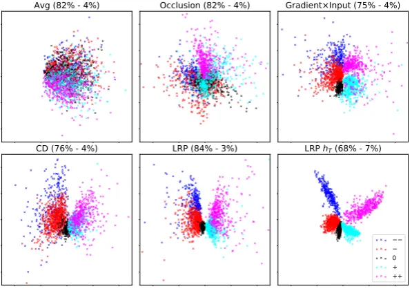
ev-ery method we report the best performing vari-ant from previous experiments, i.e.OcclusionP-diff, Gradient×Input, CD and LRP-all. Additionally we report simple averaging of word embeddings (we call itAvg). Further, for LRP, we consider an element-wise reweighting of the last time step hid-den layerhT by its relevance, since LRP delivers also a relevance for each intermediate neuron (we call it LRPhT). We also tried usinghT directly: this gave us a visualization similar toAvg. The re-sulting 2D whitened PCA projections of the test set sentences are shown in Fig.1.
Qualitatively LRP delivers the most structured representations, although for all methods the first two PCA components explain most of the data variance. Intuitively it makes also sense that the neutral sentiment is located between the positive and negative sentiments, and that the very nega-tive and very posinega-tive sentiments depart from their lower counterparts in the same vertical direction.
The advantage of having such regularities emerging via PCA projection, is that the sen-tence/phrase semantics might be investigated visu-ally, without requiring any nonlinear dimensional-ity reduction like t-SNE (typically used to explore the representations learned by recurrent models, e.g. inCho et al.,2014;Li et al.,2016). Such rep-resentations might also be useful in information retrieval settings, where one could retrieve
simi-12W.l.o.g. we use here the
Avg (82% - 4%) Occlusion (82% - 4%) Gradient×Input (75% - 4%)
CD (76% - 4%) LRP (84% - 3%) LRP hT (68% - 7%)
[image:8.595.150.449.63.272.2]0 + ++
Figure 1: PCA projection of sentence-level representations built on top of word embeddings that were linearly combined using their respective relevance. Avgcorresponds to simple averaging of word embeddings. For LRP
hT the last time step hidden layer was reweighted by its relevance. In parenthesis we indicate the percentage of variance explained by the first two PCA components (those that are plotted) and by the third PCA component. The resulting representations were roughly ordered (row-wise) from less structured to more structured.
lar sentences/phrases by employing standard eu-clidean distance.
4 Interpreting Single Predictions
Next, we analyze single predictions using the same task and model as in Section3.3, and illus-trate the usefulness of relevance visualization with
LRP-all, which is the method that performed well in both our previous quantitative experiments.
Semantic Composition. When dealing with real data, one typically has no ground truth rel-evance available. And the visual inspection of single relevance heatmaps can be counter-intuitive for two reasons: the relevance is not accurately reflecting the reasons for the classifier’s decision (the explanation method is bad), or the classi-fier made an error (the classiclassi-fier doesn’t work as expected). In order to avoid the latter as much as possible, we automatically constructed bigram and trigram samples, which are builtsolely upon the classifier’s predicted class, and visualize the resulting average relevance heatmaps for differ-ent types of semantic compositions in Table 4. For more details on how these samples were con-structed we refer to the Appendix, note though that in our heatmaps the negation<not>, the intensi-fier<very>and the sentiment words act as place-holders for words with similar meanings, since the representative heatmaps were averaged over
sev-eral samples. In these heatmaps one can see that, to transform a positive sentiment into a negative one, the negation is predominantly colored as red, while the sentiment word is highlighted in blue, which intuitively makes sense since the explana-tion is computedtowardsthe negative sentiment, and in this context the negation is responsible for the sentiment prediction. For sentiment intensifi-cation, we note that the amplifier gets a relevance of the same sign as the amplified word, indicat-ing the amplifier is supportingthe prediction for the considered target class, but still has less im-portance for the decision than the sentiment word itself (deep red colored). Both previous identified patterns also reflect consistently in the case of a negated amplified positive sentiment.
in-Composition Predicted Heatmap Relevance # samples
[image:9.595.86.513.63.133.2]1. “negated positive sentiment” − <not> <good> 2.50.3 -1.40.5 213 2. “amplified positive sentiment” ++ <very> <good> 1.10.3 4.50.7 347 3. “amplified negative sentiment” −− <very> <bad> 0.80.2 4.30.6 173 4. “negated amplified positive sentiment” − <not> <very> <good> 2.740.54 -0.340.17 -2.000.40 1745
Table 4: Typical heatmaps for various types of semantic compositions (indicated in first column), computed with the LRP-allmethod. The LSTM’s predictedclass (second column) is used as thetargetclass. The remaining columns contain the average heatmap (positive relevance is mapped to red, negative to blue, and the color intensity is normalized to the maximum absolute relevance), the corresponding word relevance mean (and std as subscript), and the number of bigrams (resp. trigrams) considered for each type of composition.
No Predicted Heatmap
1 −− it never fails to engage us .
1a + engages us .
1b − never engages us .
1c −− fails to engage us .
2 ++ ecks this one off your must-see list .
2a ++ a must-see film .
2b −− neither a must-see film .
2c ++ never a must-see film .
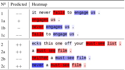
Table 5: Misclassified test sentences (1 and 2), and manually constructed sentences (1a-c, 2a-c). The LSTM’spredictedclass (second column) is used as the
targetclass for theLRP-allheatmaps.
volved in semantic composition, and that the clas-sifier might also exhibit a bias towards the types of constructions it was trained on, which might then feel more “probable” or “understandable” to him.
Besides, during our experimentations, we em-pirically found that the LRP-all explanations are more helpful when using the classifier’spredicted
class as thetarget class (rather than the sample’s
trueclass), which intuitively makes sense since it’s the class the model is the most confident about. Therefore, to understand the classification of sin-gle samples, we generally recommend this setup.
5 Conclusion
In our experiments with standard LSTMs, we find that the LRP rule for multiplicative connections introduced inArras et al. (2017b) performs con-sistently better than other recently proposed rules, such as the one fromDing et al.(2017). Further, our comparison using a 5-class sentiment predic-tion task highlighted that LRP is not equivalent to
Gradient×Input(as sometimes inaccurately stated in the literature, e.g. in Shrikumar et al., 2017) and is more selective than the latter, which is consistent with findings of Poerner et al. (2018).
Indeed, the equivalence betweenGradient×Input
and LRP holds only if using the -rule with no stabilizer ( = 0), and if the network contains
only ReLU activations and max pooling as non-linearities (Kindermans et al., 2016; Shrikumar et al.,2016). When using other LRP rules, or if the network contains other activations or product non-linearities (such as this is the case for LSTMs), then the equivalence does not hold (seeMontavon et al.(2018) for a broader discussion).
Besides, we discovered that a few methods such as Occlusion (Li et al., 2017) and CD (Murdoch et al., 2018) are not reliable and get inconsistent results on a simple toy task using an LSTM with onlyonehidden unit.
In the future, we expect decomposition-based methods such as LRP to be further useful to an-alyze character-level models, to explore the role of single word embedding dimensions, and to dis-cover important hidden layer neurons. Compared to attention weights (such as Bahdanau et al.,
2015;Xu et al.,2015;Osman and Samek,2019), decomposition-based explanations take into ac-count all intermediate layers of the neural network model, and can be related to a specific class.
Acknowledgments
[image:9.595.74.274.222.334.2]References
Julius Adebayo, Justin Gilmer, Michael Muelly, Ian Goodfellow, Moritz Hardt, and Been Kim. 2018.
Sanity Checks for Saliency Maps. In Advances in
Neural Information Processing Systems 31 (NIPS), pages 9505–9515.
Guillaume Alain and Yoshua Bengio. 2017. Under-standing intermediate layers using linear classifier
probes. In International Conference on Learning
Representations - Workshop track (ICLR).
Afra Alishahi, Grzegorz Chrupala, and Tal Linzen. 2019. Analyzing and Interpreting Neural Networks for NLP: A Report on the First BlackboxNLP Work-shop.arXiv:1904.04063. Version 1.
Marco Ancona, Enea Ceolini, Cengiz ¨Oztireli, and Markus Gross. 2018. Towards better understanding of gradient-based attribution methods for deep neu-ral networks. InInternational Conference on Learn-ing Representations (ICLR).
Jose A. Arjona-Medina, Michael Gillhofer, Michael Widrich, Thomas Unterthiner, Johannes Brand-stetter, and Sepp Hochreiter. 2018.
RUD-DER: Return Decomposition for Delayed Rewards.
arXiv:1806.07857. Version 2.
Leila Arras, Franziska Horn, Gr´egoire Montavon, Klaus-Robert M¨uller, and Wojciech Samek. 2016.
Explaining Predictions of Non-Linear Classifiers in NLP. InProceedings of the 2016 ACL Workshop on Representation Learning for NLP (Rep4NLP), pages 1–7. Association for Computational Linguistics.
Leila Arras, Franziska Horn, Gr´egoire Montavon, Klaus-Robert M¨uller, and Wojciech Samek. 2017a.
”What is relevant in a text document?”: An
inter-pretable machine learning approach. PLoS ONE,
12(8):e0181142.
Leila Arras, Gr´egoire Montavon, Klaus-Robert M¨uller, and Wojciech Samek. 2017b. Explaining Recur-rent Neural Network Predictions in Sentiment Anal-ysis. InProceedings of the 2017 EMNLP Workshop on Computational Approaches to Subjectivity, Sen-timent and Social Media Analysis (WASSA), pages 159–168. Association for Computational Linguis-tics.
Sebastian Bach, Alexander Binder, Gr´egoire Mon-tavon, Frederick Klauschen, Klaus-Robert M¨uller, and Wojciech Samek. 2015. On Pixel-Wise Ex-planations for Non-Linear Classifier Decisions by
Layer-Wise Relevance Propagation. PLoS ONE,
10(7):e0130140.
David Baehrens, Timon Schroeter, Stefan Harmel-ing, Motoaki Kawanabe, Katja Hansen, and Klaus-Robert M¨uller. 2010. How to Explain
Individ-ual Classification Decisions. Journal of Machine
Learning Research (JMLR), 11:1803–1831.
Dzmitry Bahdanau, Kyunghyun Cho, and Yoshua Ben-gio. 2015. Neural Machine Translation by Jointly
Learning to Align and Translate. InInternational
Conference on Learning Representations (ICLR).
Yonatan Belinkov and James Glass. 2019. Analysis
Methods in Neural Language Processing: A Survey.
Transactions of the Association for Computational Linguistics, 7:49–72.
Jianbo Chen, Le Song, Martin Wainwright, and Michael Jordan. 2018. Learning to Explain: An Information-Theoretic Perspective on Model Inter-pretation. InProceedings of the 35th International Conference on Machine Learning (ICML), pages 883–892.
Kyunghyun Cho, Bart van Merrienboer, Caglar Gul-cehre, Dzmitry Bahdanau, Fethi Bougares, Hol-ger Schwenk, and Yoshua Bengio. 2014. Learn-ing Phrase Representations usLearn-ing RNN Encoder-Decoder for Statistical Machine Translation. In Pro-ceedings of the 2014 Conference on Empirical Meth-ods in Natural Language Processing (EMNLP), pages 1724–1734. Association for Computational Linguistics.
Sumit Chopra, Michael Auli, and Alexander M. Rush. 2016.Abstractive Sentence Summarization with
At-tentive Recurrent Neural Networks. In
Proceed-ings of the 2016 Conference of the North American Chapter of the Association for Computational Lin-guistics: Human Language Technologies (NAACL-HLT), pages 93–98. Association for Computational Linguistics.
Joon Son Chung, Andrew Senior, Oriol Vinyals, and Andrew Zisserman. 2017. Lip Reading Sentences in
the Wild. InIEEE Conference on Computer Vision
and Pattern Recognition (CVPR), pages 3444–3453.
Misha Denil, Alban Demiraj, and Nando de Freitas. 2015.Extraction of Salient Sentences from Labelled
Documents.arXiv:1412.6815. Version 2.
Yannis Dimopoulos, Paul Bourret, and Sovan Lek. 1995. Use of some sensitivity criteria for choosing
networks with good generalization ability. Neural
Processing Letters, 2(6):1–4.
Yanzhuo Ding, Yang Liu, Huanbo Luan, and Maosong Sun. 2017. Visualizing and Understanding Neural
Machine Translation. In Proceedings of the 55th
Annual Meeting of the Association for Computa-tional Linguistics (ACL), pages 1150–1159. Associ-ation for ComputAssoci-ational Linguistics.
EU-GDPR. 2016. Regulation (EU) 2016/679 of the European Parliament and of the Council of 27 April 2016 on the protection of natural persons with re-gard to the processing of personal data and on the free movement of such data, and repealing Direc-tive 95/46/EC (General Data Protection Regulation).
Tamar Fraenkel and Yaacov Schul. 2008. The mean-ing of negated adjectives. Intercultural Pragmatics, 5(4):517–540.
Felix A. Gers, J¨urgen Schmidhuber, and Fred Cum-mins. 1999. Learning to Forget: Continual Predic-tion with LSTM. InInternational Conference on Ar-tificial Neural Networks (ICANN), volume 2, pages 850–855.
Muriel Gevrey, Ioannis Dimopoulos, and Sovan Lek. 2003. Review and comparison of methods to study the contribution of variables in artificial neural
net-work models. Ecological Modelling, 160(3):249–
264.
Fr´ederic Godin, Kris Demuynck, Joni Dambre, Wesley De Neve, and Thomas Demeester. 2018. Explaining Character-Aware Neural Networks for Word-Level
Prediction: Do They Discover Linguistic Rules? In
Proceedings of the 2018 Conference on Empirical Methods in Natural Language Processing(EMNLP), pages 3275–3284. Association for Computational Linguistics.
Klaus Greff, Rupesh K. Srivastava, Jan Koutn´ık, Bas R. Steunebrink, and J¨urgen Schmidhuber. 2017.
LSTM: A Search Space Odyssey. IEEE
Transac-tions on Neural Networks and Learning Systems, 28(10):2222–2232.
Sepp Hochreiter and J¨urgen Schmidhuber. 1996.
LSTM can Solve Hard Long Time Lag Problems. In
Advances in Neural Information Processing Systems 9 (NIPS), pages 473–479.
Sepp Hochreiter and J¨urgen Schmidhuber. 1997.
Long Short-Term Memory. Neural Computation,
9(8):1735–1780.
Alon Jacovi, Oren Sar Shalom, and Yoav Goldberg. 2018. Understanding Convolutional Neural Net-works for Text Classification. InProceedings of the 2018 EMNLP Workshop BlackboxNLP: Analyzing and Interpreting Neural Networks for NLP, pages 56–65. Association for Computational Linguistics.
´
Akos K´ad´ar, Grzegorz Chrupala, and Afra Alishahi. 2017. Representation of Linguistic Form and
Func-tion in Recurrent Neural Networks. Computational
Linguistics, 43(4):761–780.
Andrej Karpathy and Li Fei-Fei. 2015. Deep visual-semantic alignments for generating image
descrip-tions. InIEEE Conference on Computer Vision and
Pattern Recognition (CVPR), pages 3128–3137.
Pieter-Jan Kindermans, Kristof Sch¨utt, Klaus-Robert M¨uller, and Sven D¨ahne. 2016. Investigating the in-fluence of noise and distractors on the interpretation of neural networks.arXiv:1611.07270. Version 1.
Yair Lakretz, Germ´an Kruszewski, Th´eo Desbordes, Dieuwke Hupkes, Stanislas Dehaene, and Marco
Baroni. 2019. The Emergence of Number and
Syn-tax Units in LSTM Language Models. In
Proceed-ings of the 2019 Conference of the North American Chapter of the Association for Computational Lin-guistics: Human Language Technologies (NAACL-HLT), pages 11–20. Association for Computational Linguistics.
Will Landecker, Michael D. Thomure, Lu´ıs M. A. Bet-tencourt, Melanie Mitchell, Garrett T. Kenyon, and Steven P. Brumby. 2013. Interpreting Individual
Classifications of Hierarchical Networks. In IEEE
Symposium on Computational Intelligence and Data Mining (CIDM), pages 32–38.
Sebastian Lapuschkin, Alexander Binder, Gr´egoire Montavon, Klaus-Robert M¨uller, and Wojciech Samek. 2016. Analyzing Classifiers: Fisher Vectors
and Deep Neural Networks. InIEEE Conference on
Computer Vision and Pattern Recognition (CVPR), pages 2912–2920.
Sebastian Lapuschkin, Stephan W¨aldchen, Alexander Binder, Gr´egoire Montavon, Wojciech Samek, and Klaus-Robert M¨uller. 2019. Unmasking Clever Hans Predictors and Assessing What Machines Re-ally Learn.Nature Communications, 10:1096.
Quoc V. Le, Navdeep Jaitly, and Geoffrey E. Hinton. 2015. A Simple Way to Initialize Recurrent Net-works of Rectified Linear Units. arXiv:1504.00941. Version 2.
Jiwei Li, Xinlei Chen, Eduard Hovy, and Dan Juraf-sky. 2016. Visualizing and Understanding Neural
Models in NLP. In Proceedings of the 2016
Con-ference of the North American Chapter of the Asso-ciation for Computational Linguistics: Human Lan-guage Technologies (NAACL-HLT), pages 681–691. Association for Computational Linguistics.
Jiwei Li, Will Monroe, and Dan Jurafsky. 2017. Un-derstanding Neural Networks through Representa-tion Erasure. arXiv:1612.08220. Version 3.
Tal Linzen, Emmanuel Dupoux, and Yoav Goldberg. 2016. Assessing the Ability of LSTMs to Learn Syntax-Sensitive Dependencies.Transactions of the Association for Computational Linguistics, 4:521– 535.
Scott M. Lundberg and Su-In Lee. 2017. A Unified Approach to Interpreting Model Predictions. In Ad-vances in Neural Information Processing Systems 30 (NIPS), pages 4765–4774.
James Martens and Ilya Sutskever. 2011. Learning Recurrent Neural Networks with Hessian-Free Op-timization. InProceedings of the 28th International Conference on Machine Learning (ICML), pages 1033–1040.
Gr´egoire Montavon, Sebastian Lapuschkin, Alexander Binder, Wojciech Samek, and Klaus-Robert M¨uller. 2017. Explaining nonlinear classification decisions
with deep Taylor decomposition. Pattern
Gr´egoire Montavon, Wojciech Samek, and Klaus-Robert M¨uller. 2018. Methods for interpreting and
understanding deep neural network. Digital Signal
Processing, 73:1–15.
Ari S. Morcos, David G.T. Barrett, Neil C. Rabinowitz, and Matthew Botvinick. 2018. On the importance of single directions for generalization. InInternational Conference on Learning Representations (ICLR).
W. James Murdoch, Peter J. Liu, and Bin Yu. 2018.
Beyond Word Importance: Contextual Decomposi-tion to Extract InteracDecomposi-tions from LSTMs. In Inter-national Conference on Learning Representations (ICLR).
Dong Nguyen. 2018. Comparing Automatic and Hu-man Evaluation of Local Explanations for Text Clas-sification. InProceedings of the 2018 Conference of the North American Chapter of the Association for Computational Linguistics: Human Language Tech-nologies (NAACL-HLT), pages 1069–1078. Associ-ation for ComputAssoci-ational Linguistics.
Ahmed Osman and Wojciech Samek. 2019. DRAU: Dual Recurrent Attention Units for Visual Question
Answering. Computer Vision and Image
Under-standing.
Nina Poerner, Hinrich Sch¨utze, and Benjamin Roth. 2018. Evaluating neural network explanation meth-ods using hybrid documents and morphosyntactic agreement. InProceedings of the 56th Annual Meet-ing of the Association for Computational LMeet-inguis- Linguis-tics (ACL), pages 340–350. Association for Compu-tational Linguistics.
Marco Tulio Ribeiro, Sameer Singh, and Carlos Guestrin. 2016. ”Why Should I Trust You?”: Ex-plaining the Predictions of Any Classifier. In Pro-ceedings of the 22nd ACM SIGKDD International Conference on Knowledge Discovery and Data Min-ing, pages 1135–1144.
Tim Rockt¨aschel, Edward Grefenstette, Karl Moritz Hermann, Tomas Kocisky, and Phil Blunsom. 2016.
Reasoning about Entailment with Neural Attention.
InInternational Conference on Learning Represen-tations (ICLR).
Wojciech Samek, Alexander Binder, Gr´egoire Mon-tavon, Sebastian Lapuschkin, and Klaus-Robert M¨uller. 2017. Evaluating the Visualization of what
a Deep Neural Network has learned. IEEE
Trans-actions on Neural Networks and Learning Systems, 28(11):2660–2673.
Mike Schuster and Kuldip K. Paliwal. 1997.
Bidirec-tional Recurrent Neural Networks. IEEE
Transac-tions on Signal Processing, 45(11):2673–2681.
Avanti Shrikumar, Peyton Greenside, and Anshul Kun-daje. 2017. Learning Important Features Through Propagating Activation Differences. InProceedings of the 34th International Conference on Machine Learning (ICML), pages 3145–3153.
Avanti Shrikumar, Peyton Greenside, Anna Shcherbina, and Anshul Kundaje. 2016. Not Just A Black Box: Interpretable Deep Learning by
Propagating Activation Differences. 1605.01713.
Version 1.
Karen Simonyan, Andrea Vedaldi, and Andrew Zis-serman. 2014. Deep Inside Convolutional Net-works: Visualising Image Classification Models and
Saliency Maps. In International Conference on
Learning Representations - Workshop track (ICLR).
Chandan Singh, W. James Murdoch, and Bin Yu. 2019.
Hierarchical interpretations for neural network
pre-dictions. InInternational Conference on Learning
Representations (ICLR).
Richard Socher, Alex Perelygin, Jean Y. Wu, Jason Chuang, Christopher D. Manning, Andrew Y. Ng, and Christopher Potts. 2013. Recursive Deep Mod-els for Semantic Compositionality Over a Sentiment
Treebank. InProceedings of the 2013 Conference
on Empirical Methods in Natural Language Pro-cessing (EMNLP), pages 1631–1642. Association for Computational Linguistics.
Jost T. Springenberg, Alexey Dosovitskiy, Thomas Brox, and Martin Riedmiller. 2015. Striving for
Simplicity: The All Convolutional Net. In
International Conference on Learning Representations -Workshop track (ICLR).
Florian Strohm and Roman Klinger. 2018. An Em-pirical Analysis of the Role of Amplifiers, Down-toners, and Negations in Emotion Classification in
Microblogs. In IEEE International Conference
on Data Science and Advanced Analytics (DSAA), pages 673–681.
Mukund Sundararajan, Ankur Taly, and Qiqi Yan. 2017.Axiomatic Attribution for Deep Networks. In
Proceedings of the 34th International Conference on Machine Learning (ICML), pages 3319–3328.
Huijuan Xu and Kate Saenko. 2016. Ask, Attend and Answer: Exploring Question-Guided Spatial
Atten-tion for Visual QuesAtten-tion Answering. InComputer
Vision - ECCV 2016, pages 451–466.
Kelvin Xu, Jimmy Ba, Ryan Kiros, Kyunghyun Cho, Aaron Courville, Ruslan Salakhutdinov, Richard Zemel, and Yoshua Bengio. 2015. Show, Attend and Tell: Neural Image Caption Generation with
Vi-sual Attention. In Proceedings of the 32nd
Inter-national Conference on Machine Learning (ICML), pages 2048–2057.
Yinchong Yang, Volker Tresp, Marius Wunderle, and Peter A. Fasching. 2018. Explaining Therapy Pre-dictions with Layer-Wise Relevance Propagation in
Neural Networks. In IEEE International
Confer-ence on Healthcare Informatics (ICHI), pages 152– 162.
Matthew D. Zeiler and Rob Fergus. 2014.
Visualiz-ing and UnderstandVisualiz-ing Convolutional Networks. In
A Appendix
A.1 Long-Short Term Memory (LSTM) model
All LSTMs used in the present work have the fol-lowing recurrence form (Hochreiter and Schmid-huber,1997;Gers et al.,1999), which is also the most commonly used in the literature (Greff et al.,
2017):
it=sigm
Wi ht−1+Ui xt+bi
ft=sigm
Wf ht−1+Uf xt+bf
ot=sigm
Woht−1+Uo xt+bo
gt=tanh
Wg ht−1+Ug xt+bg
ct=ftct−1 + itgt ht=ottanh(ct)
wherex = (x1, x2, ..., xT)is the input sequence, sigmandtanhare element-wise activations, and
is an element-wise multiplication. The matrices
W’s,U’s, and vectorsb’s are connection weights and biases, and the initial statesh0andc0are set to
zero. The resulting last time step hidden vectorhT is ultimately fed to a fully-connected linear output layer yielding a prediction vectorf(x), with one entryfc(x)per class.
The bidirectional LSTM (Schuster and Paliwal,
1997) we use for the sentiment prediction task, is a concatenation of two separate LSTM mod-els as described above, each of them taking a dif-ferent sequence of word embedding vectors as in-put. One LSTM takes as input the words in their original order, as they appear in the input sen-tence/phrase. The other LSTM takes as input the same word sequence but inreversedorder. Each of these LSTMs yields a final hidden vector, sayh→T
andh←T . The concatenation of these two vectors is then fed to a fully-connected linear output layer, retrieving one prediction scorefc(x)per class.
A.2 Layer-wise Relevance Propagation (LRP) implementation
We employ the code released by the authors (Arras et al.,2017b) (https://github.com/ ArrasL/LRP for LSTM), and adapt it to work with different LRP product rule variants.
In the toy task experiments, we didn’t find it necessary to add any stabilizing term for numer-ical stability (therefore we use = 0for all LRP
rules). In the sentiment analysis experiments, we use = 0.001 (except for the LRP-propvariant where we use= 0.2, we tried the following val-ues: [0.001, 0.01, 0.1, 0.2, 0.3, 0.4, 1.0] and took the lowest one to achieve numerical stability).
A.3 Contextual Decomposition (CD) implementation
We employ the code released by the au-thors (Murdoch et al., 2018) (https:
//github.com/jamie-murdoch/
ContextualDecomposition), and adapt
it to work with a bidirectional LSTM. We also made a slight modification w.r.t. the author’s latest available version (commit e6575aa from March 30, 2018). In particular in filesent util.py we changed line 125 to: if i>=start and i<stop, to exclude the stop index, and call the function CD with the arguments start=k andstop=k+1 to compute the relevance of the k-th input vector, or word, in the input sequence. This consistently led to better results for the CD
method in all our experiments.
A.4 Toy task setup
As an LSTM model we consider a unidirectional LSTM with a hidden layer of size one (i.e. with one memory cell ct), followed by a linear out-put layer with no bias. Since the inout-put is two-dimensional, this results in an LSTM model with 17 learnable parameters. The weights are ran-domly initialized with the uniform distribution
U(−1.0,1.0), and biases are initialized to zero. We train the model with Pytorch’s LBFGS opti-mizer, with an initial learning rate of 0.002, for 1000 optimizer steps, and reduce the learning rate by a factor of 0.95 if the error doesn’t decrease within 10 steps. We also clip the gradient norm to 5.0. With this setting around 1/2 of the trained models on addition and 1/3 of the models for sub-traction converged to a good solution with a vali-dation MSE<10−4.
A.5 Semantic composition: generation of representative samples
the considered sentiment words are clearly identi-fied by the model as being from the positive senti-ment (+), resp. the negative sentiment (−) class.
In a second step, we build a list of negations and amplifiers. To that end, we start by considering the same lists of 39 negations and 69 amplifiers as in
Strohm and Klinger(2018), from which we retain only those that are classified as neutral (class 0) by the LSTM model, which leaves us with a list of 8 negations and 29 amplifiers. This way we dis-card modifiers that are biased towards a specific sentiment, since our goal is to analyze the compo-sitional effect of modifiers.
Then, for each type of considered semantic composition (see Table 4), we generate bigrams resp. trigrams by using the previously defined lists of modifiers and sentiment words.
For compositions of type 1 (“negation of pos-itive sentiment”), we note that among the con-structed bigrams 60% are classified as nega-tive (−) by the LSTM model, 26% are predicted as neutral (0), and for the remaining 14% of bigrams the negation is not identified correctly and the cor-responding bigram is classified as positive (+). In order to remove negations that are ambiguous to the classifier, we retain only those negations which in at least 40% of the cases predict the bigram as negative. These negations are: [’neither’, ’never’, ’nobody’, ’none’, ’nor’]. Then we average the re-sults over all bigrams classified as negative (−).
For compositions of type 2 and 3 we proceed similarly. For type 2 compositions (“amplifica-tion of positive sentiment”), we note that 29% of the constructed bigrams are classified as very pos-itive (++), and for type 3 compositions (“amplifi-cation of negative sentiment”), 24% are predicted as very negative (−−), while the remaining bi-grams are of the same class as the original sen-timent word (thus the amplification is not identi-fied by the classifier). Here again we retain only unambiguous modifiers, which in at least 40% of the cases amplified the corresponding senti-ment. The resulting amplifiers are: [’completely’, ’deeply’, ’entirely’, ’extremely’, ’highly’, ’in-sanely’, ’purely’, ’really’, ’so’, ’thoroughly’, ’ut-terly’, ’very’] for type 2 compositions; and [’com-pletely’, ’entirely’, ’extremely’, ’highly’, ’really’, ’thoroughly’, ’utterly’] for type 3 compositions. Then we average the results over the correspond-ing bigrams which are predicted as very posi-tive (++), resp. very negative (−−).
For type 4 compositions (“negation of ampli-fied positive sentiment”), we construct all possi-ble trigrams with the initial lists of negations, am-plifiers and positive sentiment words. We keep for the final averaging of the results only those trigrams where both the effect of the amplifier, and of the negation are correctly identified by the LSTM model. To this end we classify the corre-sponding bigram formed by combining the ampli-fier with the positive sentiment word, and keep the corresponding sample if this bigram is predicted as very positive (++). Then we average the re-sults over trigrams predicted as negative (−) (this amounts to finally retain 1745 trigrams).