One EMU Fiscal Policy for the EURO

Munich Personal RePEc Archive

One EMU Fiscal Policy for the EURO

Cole, Alexandre Lucas and Guerello, Chiara and Traficante,

Guido

Parliamentary Budget Office, LUISS Guido Carli, European

University of Rome

2018

Online at

https://mpra.ub.uni-muenchen.de/97380/

One EMU Fiscal Policy for the EURO

Alexandre Lucas Cole†

PBO (UPB) & LUISS Guido Carli

Chiara Guerello‡

LUISS Guido Carli

Guido Traficante§

European University of Rome

October 26, 2018

Abstract

We build a Two-Country New-Keynesian DSGE model of a Currency Union to study the effects of fiscal policy coordination, by evaluating the stabilization properties and welfare implications of different fiscal policy scenarios. Our main findings are that a government spending rule which targets the net exports gap rather than the domestic output gap produces more stable dynamics and that consolidating government budget constraints across countries with symmetric tax rate movements provides greater stabilization. A key role is played by the trade elasticity which determines the impact of the terms of trade on net exports. In fact, when goods are complements, the stabilization properties of coordinating fiscal policies are no longer supported. These findings point out to possible policy prescriptions for the Euro Area: to coordinate fiscal policies by reducing international demand imbalances, either by stabilizing trade flows across countries or by creating some form of Fiscal Union or both.

JEL classification: E62, E63, F42, F45, E12

Keywords: Fiscal Policy, International Policy Coordination, Monetary Union, New Keynesian

∗_{Forthcoming in}

Macroeconomic Dynamics. We thank William A. Barnett (editor) and two anonymous referees for valuable comments on an earlier draft. A special thanks to Pierpaolo Benigno for useful research guidance and to Giovanna Vallanti for helpful academic guidance. We would like to thank Konstantinos Tsinikos, Pietro Reichlin, Andrea Ferrero, Tommaso Trani, Niku M¨a¨att¨anen and participants in LUISS Guido Carli seminars, the FIRSTRUN Workshop of September 26th 2016 and the 12th Dynare Conference for useful comments and suggestions. All errors are our own. The views and opinions expressed in this paper are those of the authors and do not necessarily reflect the official policy or position of any other agency, organization, employer or company. We acknowledge financial support through the research project FIRSTRUN (www.firstrun.eu) (Grant Agreement 649261) funded by the Horizon 2020 Framework Programme of the European Union.

†_{Alexandre Lucas Cole: Parliamentary Budget Office - Ufficio Parlamentare di Bilancio, via del Seminario 76,}

00186 Rome,alexcole82@gmail.com

‡_{Chiara Guerello: LUISS Guido Carli, viale Romania 32, 00197 Rome,cguerello@luiss.it}

§_{Guido Traficante: European University of Rome, via degli Aldobrandeschi 190, 00163 Rome,}

1

Introduction

Given a single monetary policy in the European Economic and Monetary Union (EMU), specific shocks cannot be addressed through monetary policy, but must be balanced by country-specific fiscal policies. Whether this calls for coordination or not is a much debated issue, and has been typically investigated by looking at fiscal multipliers, as Farhi and Werning(2012) finds a greater output multiplier if government spending is financed by a foreign country rather than the home country. This would create a scope for a central EMU budget, as centrally financed government spending has larger effects than nationally financed government spending. This was mentioned also in the more recentJuncker et al.(2015), where a Fiscal Union is seen as a Euro area-wide macroeconomic stabilization tool, over and above national fiscal policies needed to cushion country-specific shocks, which is thought to be key in avoiding procyclical fiscal policies at all times. In addition, as emphasized inForni, Gerali and Pisani(2010), a reduction in public spending followed by lower distortionary taxation can produce positive cross-country spillovers in the Euro Area. Also, from an empirical perspective Evers (2012) and Furceri and Zdzienicka (2015) show that a centralized transfer mechanism, which is based on non-regressive temporary transfers and automatic rules, could significantly increase income and consumption smoothing. However, as argued by Bargain et al. (2013), the partial (or full) replacement of the existing national system by an EU-wide integrated tax and transfer system or by a system of fiscal equalization requires to be considerable in magnitude to achieve significant income stabilization and always at the cost of significant redistributive effects.

We analyze the stabilization properties and the welfare implications from coordination, con-sidering whether there is a scope for a fiscal capacity in the EMU to address asymmetric shocks to member countries, as a shock-absorption mechanism1. We compare different scenarios for fiscal policy coordination in the EMU. First, we compare the case where each country chooses its gov-ernment consumption, transfers and taxation (Pure Currency Union) with a transfer-based Fiscal Union where the policy variables are set by the union as a whole, and with a consolidated budget and symmetric tax rate movements (Full Fiscal Union), with an intermediate case of fiscal policy coordination, where government expenditure responds to international variables (Coordinated Cur-rency Union). Second, we consider two welfare criteria, and by comparing these three scenarios, we evaluate the welfare gains from a common macroeconomic stabilization function, bringing to policy conclusions for the proper macroeconomic management of a Currency Union.

Our approach is similar to the open economy of Gal´ı(2009), but in a two-country setting like

inSilveira(2006)2_{. Our model follows mainly the specifications ofFerrero(2009), which adapts the} optimal approach ofBenigno and Woodford(2004) to monetary and fiscal policy in a cashless closed economy without capital, where there are only distortionary taxes as sources of government revenue, to a two-country open-economy Currency Union setting. We add home bias in consumption (or a degree of openness to international trade) and targeting rules for fiscal policy (following Hjortsø

(2016)). The former allows for deviations from Purchasing Power Parity, while the latter is a fiscal policy stabilization rule3.

Our model is structured to allow for spillovers from monetary to fiscal policy and viceversa, and from one country to another through country-specific fiscal policies. Nominal rigidities, in the form of staggered prices, generate real effects of monetary policy, while distortionary taxation generates non-Ricardian effects of fiscal policy. This framework allows to study the interaction between country-specific fiscal policies, where in the absence of the nominal exchange rate as an automatic stabilizer, fiscal policies influence each other through their effects on net exports and the terms of trade.

Our main findings are that coordinating fiscal policies, by targeting the net exports gap rather than the domestic output gap, produces more stable dynamics and that consolidating government budget constraints across countries with symmetric tax rate movements provides greater stabi-lization than with separate budget constraints and independent tax rate movements. In terms of policy prescriptions for the Euro Area, our findings suggest to coordinate fiscal policies by reducing international demand imbalances, either by stabilizing trade flows across countries or by creating some form of Fiscal Union or both.

Differently from previous literature, our design of a Currency Union allows to investigate jointly different phenomena which have been usually dealt with separately. On one hand, we consider endogenous fiscal targeting rules on the spending side in conjunction with distortionary taxes on the financing side, hence considering two-sided fiscal coordination. On the other hand, we consider both the case of fiscal policy coordination and of a transfer union as nested scenarios, hence evaluating the marginal gains of increasing the level of coordination.

Our work draws on two strands of literature. The literature on Fiscal Unions is not very large, but we make use of a few contributions to motivate our analysis of a Fiscal Union inside a Currency Union, as a form of cross-country insurance to improve risk-sharing and stabilization.

von Hagen and Wyplosz (2008) finds that, in a Currency Union where fiscal policy cannot be

2_{The structure ofGal´ı and Monacelli(2008) andFarhi and Werning(2017) with a continuum of countries means}

that more variables will be exogenous, compared to a two-country model, and that a single country, being one of an infinite continuum, as specified inGal´ı(2009), does not influence any world variable. This means that all world variables must be exogenous and that it is harder to see the interaction among countries, so that international trade has no role because any expenditure on goods from any one country has a value of zero, being one of infinitely many composing the integral, as written inGal´ı(2009) that an integral of any variable over all countries is the same as an integral of the same variable over all countries except one. This poses questions on the validity of such a model and pushes us to prefer a two-country model instead, where the interactions among the two countries (or two groups of countries) are more evident and the dynamics are thus clearer.

3_{A similar model to ours is the Currency Union model ofBenigno(2004), but without a fiscal authority and with}

countercyclical, a collective insurance system is needed in place of external borrowing and lending, and this is preferable in the form of tax revenue sharing (a form of fiscal or transfer union).

Dmitriev and Hoddenbagh (2015) also shows that welfare gains from an optimal Fiscal Union inside a Currency Union are greater with incomplete financial markets, although there is still a gain with complete markets. Farhi and Werning(2017) finds instead that a fiscal or transfer union is needed, also in the presence of complete international financial markets, because a Currency Union prevents monetary policy from stabilizing asymmetric shocks, thus giving a stabilization role to fiscal policy. In line with this literature, we show that, even when financial markets are fully integrated, consolidating budget constraints across countries with symmetric tax rate movements provides greater stabilization than with separate budget constraints. We specifically show that in the case of a constrained debt policy (balanced budget), a transfer union stabilizes the economy by allowing for a greater fiscal capacity where needed.

The relevance of cross-country imbalances in net exports and the impact of coordinated fiscal policies for the transmission of shocks across countries has been largely debated in the literature.

Mink, Jacobs and de Haan (2016) shows that output growth differentials in the euro area are relatively lower than trade imbalances. Moreover, these trade imbalances have not decreased sig-nificantly since the introduction of the Euro. Canova, Ciccarelli and Dallari (2013) shows that the transmission of asymmetric shocks on output in both countries depends mainly on the dynam-ics of the trade balance, which in turn depend strongly on imports. Additionally, Beetsma and Jensen(2005) shows that, while optimal monetary policy is exclusively concerned with stabilizing the union-wide economy, optimal coordinated fiscal policy focuses entirely on the stabilization of relative inflation and the terms of trade. Hebous and Zimmermann (2013) shows empirically the importance of coordinating fiscal stimuli because of the greater uncontrolled impact of asymmetric fiscal stimuli.

The remainder of the paper is structured as follows. Section 2 describes the general model and the fiscal policy scenarios of a Pure Currency Union, a Coordinated Currency Union and a Full Fiscal Union. Section 3 presents the calibration of the parameters and steady state stances of the model to two groups of countries in the EMU. Section 4 provides numerical simulations under different scenarios, comparing different degrees of fiscal policy coordination and alternative government financing schemes. Section 5 describes two welfare criteria and provides welfare rank-ings of the different fiscal policy scenarios. Section 6 collects the main conclusions and provides possible extensions. Appendix A.1 provides all the equilibrium conditions of the model used for the simulations, while Appendix A.2 describes the steady state on which the model is calibrated. Appendix A.3 shows numerical simulations and welfare evaluations of the case for international goods as complements, rather than substitutes.

2

A Two-Country Currency Union Model

The world economy is composed of two countries (or groups of countries), which form a Currency Union. Both economies are assumed to share identical preferences, technology and market structure, but may be subject to different shocks, and have different price rigidities, initial conditions and fiscal stances. The two countries are indexed by H and F for Home and Foreign. The world is populated by a continuum of infinitely-lived households of measure one, indexed byi∈[0,1]. Each household owns a monopolistically competitive firm producing a differentiated good, indexed by

j∈[0,1]. The population on the segment [0, h) belongs to country H while the population on the segment [h,1] belongs to country F. This means that the relative size of country H is h ∈ [0,1], while the relative size of country F is 1−h. This is true for both households and firms. The economy is a cashless one.

Firms set prices in a staggered fashion following Calvo (1983) and use only labour for produc-tion. There is no capital and no investment. Labour markets are competitive and internationally segmented, so that labour supply is country-wide and not firm-specific. All goods are tradable and the Law of One Price (LOP) holds for all single goods j. At the same time deviations from Purchasing Power Parity (PPP) may arise because of home bias in consumption. Financial markets are complete internationally, allowing households to trade a full set of one-period state-contingent claims across borders, and also trade internationally one-period risk-free bonds issued by the two countries’ governments, which are perfect substitutes, offering the same return. FollowingFarhi and Werning(2017) we view the complete financial markets’ assumption as a useful one to highlight the fact that any inefficiency in private insurance, and consequent gain from government intervention, does not arise from inefficiency in financial markets4_.

Each country has an independent Fiscal Authority, while the Currency Union shares a common Monetary Authority. The Central Bank sets the nominal interest rate for the whole Currency Union following an Inflation Targeting regime, where the target is on union-wide CPI inflation. We

4_{Furthermore, we view complete financial markets as the goal of financial market integration for the European}

assume that both countries must follow a balanced budget fiscal policy. In particular, governments choose the level of public consumption and transfers, which are financed by distortionary taxes on labour income and firm sales and eventually by short-term government bonds, although keeping real government debt constant. In this setup, balanced budget constraints are neither redundant nor an alternative to fiscal coordination, as monetary policy affects fiscal policies, other than fiscal policies influencing each other. Therefore, we design both revenue-based fiscal constraints and different degrees of fiscal policy coordination on both the revenue and expenditure side. Fiscal policy is designed following the Fiscal Compact Rules, by imposing balanced budget policies, as it is one of the goals of a fully integrated Currency Union.

In what follows we denote variables referred to the Foreign country with a star (∗) and, given symmetry between the two countries, we show the main equations only for country H, while we show the equations for country F only when they are very different from those for country H.

2.1 Households

In each country there is a continuum of households, which gain utility from private consumption and disutility from labour, consume goods produced in both countries with home bias, supply labour to domestic firms and collect profits from those firms. Households can trade a complete set of one-period state-contingent claims across borders and also trade internationally one-period risk-free bonds issued by the two countries’ governments (which are perfect substitutes and so offer the same return), subject to their budget constraint.

Each household in country H, indexed byi∈[0, h), seeks to maximize the present-value utility5:

E0 ∞ X

t=0

βtξt

(Ci

t)1−σ−1

1−σ −

(Ni t)1+ϕ

1 +ϕ

(2.1.1)

whereβ∈[0,1] is the common discount factor, which households use to discount future utility,σ is the inverse of the elasticity of intertemporal substitution6 (it is also the Coefficient of Relative Risk Aversion (CRRA)),ϕis the inverse of the Frisch elasticity of labour supply7, andξt is a preference

shock toHome households. This preference shock is assumed to follow the AR(1) process in logs:

ξt= (ξt−1)ρξeεξ,t (2.1.2)

whereρξ∈[0,1] is a measure of persistence of the shock andεξ,tis a zero mean white noise process.

Ni

t denotes hours of labour supplied by households in country H.Cti is a composite index for private

5_{We choose to specify additively separable period utility of the type with Constant Relative Risk Aversion}

(CRRA), so with constant elasticity of intertemporal substitution, and with constant elasticity of labour supply.

6_{The elasticity of intertemporal substitution measures the responsiveness of consumption growth to changes in}

the real interest rate, which is the relative price of consumption between different dates, and is defined as the percent change in consumption growth divided by the percent change in the gross real interest rate.

7_{The Frisch elasticity of labour supply measures the extent to which labour supply responds to a change in the}

consumption defined by:

C_ti ≡h(1−α)1η_(Ci

H,t)

η−1

η _+α

1

η_(Ci

F,t)

η−1

η

i η η−1

(2.1.3)

for households in country H, whereC_H,ti is an index of consumption of domestic goods for households in country H, given by the constant elasticity of substitution (CES) function (also known asDixit and Stiglitz(1977) aggregator function):

C_H,ti ≡ 1

h

1

ε Z h

0

C_H,ti (j)ε−1ε dj

! ε ε−1

(2.1.4)

wherej∈[0,1] denotes a single good variety of the continuum of differentiated goods produced in the world economy. Ci

F,t is an index of consumption of imported goods for households in country

H, given by the analogous CES function:

C_F,ti ≡ 1

1−h

1

εZ 1

h

C_F,ti (j)ε−1ε dj

! ε ε−1

(2.1.5)

The parameter ε >1 measures the elasticity of substitution between varieties produced within a given country. The parameterη >0 measures the substitutability between domestic and foreign goods (international trade elasticity). The parameter α ∈ [0,1] is a measure of openness of the

Home economy to international trade. Equivalently (1−α) is a measure of the degree of home bias in consumption in country H. When α tends to zero the share of foreign goods in domestic consumption vanishes and the country ends up in autarky, consuming only domestic goods. If 1−α > h there is home bias in consumption in country H, because the share of consumption of domestic goods is greater than the share of production of domestic goods.

Households in country H maximize their present-value utility, equation 2.1.1, subject to the following sequence of budget constraints:

Z h

0

PH,t(j)CH,ti (j)dj+

Z 1

h

PF,t(j)CF,ti (j)dj+Dit+Bti ≤

Di t−1

Qt−1,t

+B_ti₋₁(1+it−1)+(1−τtw)WtNti+Tti+Γit

(2.1.6) for t = 0,1,2, . . ., where PH,t(j) is the price of domestic variety j, PF,t(j) is the price of variety

j imported from country F, Di

t−1 is the portfolio of state-contingent claims purchased by the household in periodt−1,Qt−1,t is the stochastic discount factor, which is the same for households

in both countries and represents the price of state-contingent claims or equivalently the inverse of the gross return on state-contingent claims,Bi

t−1 are risk-free government bonds (of either or both governments) purchased by the household in periodt−1, it−1 is the nominal interest rate set by the central bank in period t−1, which is also the net return on both government bonds,Wt is the

nominal wage for households in country H,Ti

t denotes lump-sum transfers from the government to

households, Γi

τw

t ∈[0,1] is a marginal tax rate on labour income paid by households to the government.

All variables are expressed in units of the union’s currency. Last but not least, households in country H are subject to the following solvency constraint, for all t, that prevents them from engaging in Ponzi-schemes:

lim

T→∞Et

Qt,TDiT ≥0 (2.1.7)

Aggregating the intratemporal optimality condition yields the aggregate labour supply equation for households in country H:

Nt= (h)1+

σ ϕ(C_t)−

σ ϕ

(1−τ_tw)Wt

Pt

1

ϕ

(2.1.8)

where Nt is aggregate labour supply and Ct is aggregate consumption for households in country

H, while aggregating the intertemporal optimality condition for households in country H, taking conditional expectations and using the no-arbitrage condition between government bonds and state-contingent claims, yields:

1 1 +it

=Et{Qt,t+1}=βEt

(

ξt+1

ξt

Ct+1

Ct

−σ

1 Πt+1

)

(2.1.9)

where ₁₊1_i

t =Et{Qt,t+1}is the price of a one-period riskless government bond paying off one unit

of the union’s currency int+ 1 and Πt+1 ≡ P_Pt+1_t is gross CPI inflation in country H. The Consumer Price Index (CPI) for country H is given by:

Pt≡

(1−α)(PH,t)1−η+α(PF,t)1−η

1

1−η _(2.1.10)

where PH,t is the domestic price index or Producer Price Index (PPI) in country H and PF,t is a

price index for goods imported from country F, respectively defined by:

PH,t≡

1

h

Z h

0

PH,t(j)1−εdj

1 1−ε

(2.1.11)

PF,t≡

1 1−h

Z 1

h

PF,t(j)1−εdj

1 1−ε

(2.1.12)

2.2 International Identities and Assumptions

Several international identities and assumptions need to be spelled out in order to link the Home

economy to theForeign one and to be able to close the model.

The terms of trade are defined as the price of foreign goods in terms of home goods, for house-holds in country H and in country F, and are given respectively by:

St≡

PF,t

PH,t

and St∗≡

P_F,t∗ P∗

H,t

Given the previous definition, an increase in the terms of trade is equivalent to a deterioration of the terms of trade, because imports become more expensive compared to exports.

Although deviations from Purchasing Power Parity (PPP)may arise because of home bias in consumption, we assume that the Law of One Price (LOP) holds for every single good j, which implies:

PH,t(j) =PF,t∗ (j) and PF,t(j) =PH,t∗ (j) (2.2.2)

for all j∈[0,1], wherePH,t(j) (or PF,t(j) for goods imported from country F) is the price of good

j in country H andP_F,t∗ (j) (or P_H,t∗ (j) for goods produced in country F) is the price of good j in country F in terms of the union’s currency. Plugging the previous expressions into the definitions of PH,t and PF,t and combining them with the definition of the terms of trade for countries H and

F yields:

St=

PF,t

PH,t

= P

∗

H,t

P∗

F,t

= 1

S∗

t

(2.2.3)

The relationship between PPI inflation and CPI inflation in country H is given by:

Πt= ΠH,t

1−α+α(St)1−η

1−α+α(St−1)1−η 1

1−η

(2.2.4)

while dividing the terms of trade in periodtby the terms of trade in periodt−1 yields a relationship showing the evolution of the terms of trade over time:

St

St−1

= ΠF,t ΠH,t

= Π

∗

H,t

ΠH,t

=⇒ St=

Π∗_H,t ΠH,t

St−1 (2.2.5)

as a function of PPI inflation in both countries H and F.

The Real Exchange Rate between the Home country and country F is the ratio of the two countries’ CPIs, expressed both in terms of the union’s currency, and is defined by:

Qt≡

P_t∗ Pt

=St

1−α∗+α∗(St)η−1

1−α+α(St)1−η

1 1−η

(2.2.6)

where the difference between the real exchange rate and the terms of trade is given by the degree of openness of the two countries and the international trade elasticity. Given the previous definition, as for the terms of trade, an increase in the real exchange rate is equivalent to a deterioration of the real exchange rate. If the countries both have complete home bias (α = α∗ _{= 0), then they} resemble closed economies and the real exchange rate is exactly equal to the terms of trade, because the CPI and PPI are equal to each other in each country.

Figure 1: Elasticity of the Real Exchange Rate to the Terms of Trade as a function of Trade Openness

0 0.2 0.4 0.6

0.8 1 1.2 1.4

1.6 1.8 2 0

0.2 0.4 0.6 0.8 1

0 0.5 1 1.5 2

Real Exchange Rate Elasticty to Terms of Trade

Terms of Trade Trade Openess

R

ea

l E

xc

ha

ng

e

R

at

e

0.2 0.4 0.6 0.8 1 1.2 1.4 1.6 1.8

home bias. As Figure 1 shows, the real exchange rate appreciates as the terms of trade increase if there is home bias in consumption in country H (1−α > h), while the real exchange rate depreciates when the terms of trade increase otherwise. Notice that this is the case for our calibration (see Section3), where we have 1−α = 0.48> h= 0.4. This condition implies that there is home bias in consumption also in country F (1−α∗ _{>1−h) for the real exchange rate to appreciate as the} terms of trade increase, and viceversa otherwise.

Since one-period state-contingent claims can be traded freely between households within and across borders, they are in zero international net supply, so that the market clearing condition for these assets in every period tis consequently given by:

Z h

0

D_tidi+ Z 1

h

D_t∗idi=hDi_t+ (1−h)D_t∗i =Dt+D∗t = 0 (2.2.7)

exports minus imports, and for country H are given in real terms (divided byPH,t) by:

g

N Xt=Yt−

Pt

PH,t

Ct−Gt=Yt−

1−α+α(St)1−η

1

1−η_C

t−Gt (2.2.8)

where net exports are shown to be a function of the country’s degree of openness and the terms of trade, other than domestic production and public and private domestic consumption.

Since exports for country H are imports for country F and viceversa, then net exports are in zero international net supply. In real terms: N Xgt+StN Xg

∗

t = 0.

Net Foreign Assets are given by the sum of private and public assets held abroad, and for country H are given in real terms (divided byPH,t) by:

^

N F At≡D˜t+ ˜Bt−B˜tG (2.2.9)

Since foreign assets for country H are domestic assets for country F, then net foreign assets are in zero international net supply. In real terms: N F A^t+StN F A^

∗

t = 0.

From the households’ budget constraint, substituting in firm profits, labour income, the ex-pression for transfers backed out from the government budget constraint and the definitions of net exports and net foreign assets, yields the following relationship between net foreign assets and net exports in real terms (divided by PH,t) for country H:

^

N F At= (1 +it−1)

^

N F At−1 ΠH,t

+N Xgt (2.2.10)

2.3 Firms

In country H there is a continuum of firms indexed by j ∈ [0, h) each producing a differentiated good with the same technology represented by the following production function:

Yt(j) =AtNt(j) (2.3.1)

where At represents the level of technology in country H, which evolves exogenously over time

following the AR(1) process in logs:

At= (At−1)ρaeεa,t (2.3.2)

whereρa∈[0,1] is a measure of persistence of the shock andεa,tis a zero mean white noise process.

From the production function we can derive labour demand for individual firms in country H and the respective real marginal costs of production, which are equal across firms in each country and are given by:

M Ct=

Wt

AtPH,t

(2.3.3)

demand for country H:

Nt≡

Z h

0

Nt(j)dj =

Z h

0

Yt(j)

At

dj = Yt

At Z h 0 1 h

PH,t(j)

PH,t

−ε

dj = Yt

At

dt (2.3.4)

whereYt is aggregate output in country H, given by:

Yt≡

1

h

1

ε Z h

0

Yt(j)

ε−1

ε dj

! ε ε−1

(2.3.5)

and where the term:

dt≡

Z h

0 1

h

PH,t(j)

PH,t

−ε

dj (2.3.6)

represents relative price dispersion across firms in country H. In steady state and in a flexible price equilibrium relative price dispersion is equal to one.

Aggregating over all j∈[0, h) firmj’s periodtprofits net of taxes in country H, substituting in labour demand, marginal costs, the demand function for output, using the definition of PH,t, and

substituting in price dispersion yields aggregate profits net of taxes in country H:

Γt= (1−τts)PH,tYt−PH,tM CtYtdt=PH,tYt(1−τts−M Ctdt) (2.3.7)

whereτts is the marginal tax rate on firm sales in country H.

FollowingCalvo(1983), each firm in country H may reset its price with probability 1−θin any given period. Thus, each period a fraction 1−θ of randomly selected firms reset their price, while a fraction θ keep their prices unchanged. As a result, the average duration of a price in country H is given by (1−θ)−1_{, andθ can be seen as a natural index of price stickiness for country H. In} country F each firm may reset its price with probability 1−θ∗ in any given period. This allows for the two countries to have different degrees of price rigidity.

A firm in country H re-optimizing in periodtwill choose the price ¯PH,t that maximizes the

cur-rent market value of the profits net of taxes generated while that price remains effective. Formally, it solves the problem:

max ¯ PH,t ∞ X k=0

θkEt

Qt,t+kYt+k|t(j)

(1−τ_ts_+k) ¯PH,t−M Ctn+k (2.3.8)

subject to the sequence of demand constraints8:

Yt+k|t(j) =

_¯

PH,t

PH,t+k

−ε

Yt+k

h (2.3.9)

8_{The derivation of the demand function for firms is much like the derivation of the demand function for}

con-sumption goods, except for the timing of price setting, which implies thatPH,t+k(j) = ¯PH,t(j) with probabilityθk

for k = 0,1,2, . . ., where Qt,t+k is the households’ stochastic discount factor in country H for

discounting k-period ahead nominal payoffs from ownership of firms, defined by:

Qt,t+k=βk

ξt+k

ξt

Ct+k

Ct

−σ

Pt

Pt+k

(2.3.10)

for k= 0,1,2, . . ., and where Yt+k|t(j) is the output in period t+k for firm j which last reset its

price in periodt.

The optimal price chosen by firms in country H can be expressed as a function of only aggregate variables:

¯

PH,t=

ε ε−1

P∞

k=0(βθ)kEt

n_ξ

t+k(Ct+k)−σ

Pt+k

Yt+k

(PH,t+k)−εM C

n t+k

o

P∞

k=0(βθ)kEt

n_ξ

t+k(Ct+k)−σ

Pt+k

Yt+k

(PH,t+k)−ε(1−τ

s t+k)

o (2.3.11)

Notice that in the zero inflation steady state and in the flexible price equilibrium the previous equation simplifies to:

¯

PH =

ε

(ε−1)(1−τs₎M C

n _(2.3.12)

where M Cn _{is the nominal marginal cost in steady state and in the flexible price equilibrium in}

country H, and where the optimal price is shown to be set as a markup over nominal marginal costs.

2.4 Central Bank and Monetary Policy

The only central bank in the Currency Union sets monetary policy by choosing the nominal interest rate to target union-wide inflation through a Taylor rule. We assume that the central bank cares only about inflation, as price stability is the primary objective of the ECB.

Monetary policy follows an Inflation Targeting regime of the kind:

β(1 +it) =

ΠU

t

ΠU

φπ(1−ρi)

[β(1 +it−1)]ρi (2.4.1)

where union-wide inflation is defined as the population-weighted geometric average of the CPI inflation in the two countries:

ΠU_t ≡(Πt)h(Π∗t)1−h (2.4.2)

while variables without subscripts t denote their respective steady state levels, φπ represents the

responsiveness of the interest rate to inflation andρi is a measure of the persistence of the interest

rate over time (interest rate smoothing).

2.5 Fiscal Policy and Coordination

to fiscal coordination, as monetary policy affects fiscal policy, other than fiscal policies influencing each other. Therefore we design both revenue based fiscal constraints and different degrees of fiscal policy coordination.

Pure Currency Union The first scenario is a Pure Currency Union (uncoordinated fiscal pol-icy), where each government chooses the amount of government consumption and transfers for domestic stabilization purposes, financed by marginal tax rates on labour income and firm sales and eventually by short-term government bonds. Since real government debt must remain constant so as to have a balanced budget, movements in government consumption and transfers are financed by movements in taxes, so as to satisfy the budget constraint. Nonetheless, since government debt is positive, monetary policy affects interest payments on that debt through its effect on the interest rate, which also must be financed by tax rate movements, so as to satisfy the budget constraint. In this case both countries manage fiscal policy independently without cooperating, because they only care about stabilizing their own domestic demand, by using government consumption and transfers to absorb excess domestic supply with respect to the steady state.

In country H the government finances a stream of public consumption Gt and transfers Tt

subject to the following sequence of budget constraints:

Z h

0

PH,t(j)Gt(j)dj+

Z h

0

T_tidi+BG_t−1(1 +it−1) =BtG+τtsPH,tYt+

Z h

0

τ_twWtNtidi (2.5.1)

where the right hand side represents government income from taxation and newly issued government bonds, while the left hand side represents total government spending on consumption and transfers, and on government bonds due at the end of periodt, including interest. BG

t are government bonds

issued by country H in period t. Government consumption, Gt, is given by the following CES

function, just like equation 2.3.9 for the demand function for firms, where we assume that the government purchases only goods produced domestically (complete home bias):

Gt≡

1

h

1

ε Z h

0

Gt(j)

ε−1

ε dj

! ε ε−1

(2.5.2)

Fiscal policy in country H chooses government consumption to stabilize the output gap coun-tercyclically through the spending rule:

Gt

G =

Yt

Y

−ψy(1−ρg)

Gt−1

G

ρg

eεtg, _(2.5.3)

so as to absorb excess domestic supply with respect to steady state, while keeping real transfers constant and balancing the budget, so as to keep real debt constant:

˜

Tt= ˜T B˜tG=

˜

B_tG₋₁

ΠH,t

which means that government spending is financed by the variation of the tax rates on labour income and firm sales from their steady state levels respectively by a share γ ∈ [0,1] and 1−γ

through the following tax rule9_:

γ(τ_ts−τs) = (1−γ)(τ_tw−τw) (2.5.5)

whereψy ≥0 represents the responsiveness of government consumption to variations of the output

gap, ρg ∈ [0,1] is a measure of persistence of the government consumption shock in its AR(1)

process in logs and εg,t is a zero mean white noise process, while variables without subscript t

represent their respective steady state level.

Since government bonds are traded freely within and across borders without frictions and are perfectly substitutable because they offer the same return, the total amount of bonds held by households in both countries must equal the total amount of bonds issued by the two countries’ governments, so that the market clearing condition for these assets in every periodtis given in real terms (divided byPH,t) by:

˜

Bt+StB˜t∗ = ˜BtG+StB˜∗tG (2.5.6)

Coordinated Currency Union If the Governments of the two countries choose to coordinate, we assume they use their fiscal instruments to target a common objective, while maintaining in-dependent budget constraints. Instead of using government consumption to stabilize the domestic output gap countercyclically, we assume that they use the same fiscal instrument to stabilize the net exports gap procyclically. This way, instead of using government consumption or transfers to ab-sorb excess domestic supply with respect to steady state, which can be also exported, they are used to absorb excess international supply (net exports) with respect to steady state. This represents the act of coordinating their policies on a common objective, which depends on the interactions between the two economies, for international rather than domestic stabilization purposes. The budget constraints of the two fiscal authorities instead remain unmodified. Here both countries still manage fiscal policy independently, but decide to coordinate by stabilizing their trade flows10. Fiscal policy in country H chooses government consumption to stabilize its real net exports gap

9_{If the overall tax rate is defined as:}

τto≡τ s t +τ

w t

then the variation of the tax rates on labour income and on firm sales will be given respectively by a shareγ∈[0,1] and 1−γof the variation of the overall tax rate in the following way:

(τtw−τ w

)≡γ(τto−τ o

)

(τts−τ s

)≡(1−γ)(τto−τ o

)

which implies the tax rule in the text.

10_{We choose the net exports gap as a common objective because one of the main concerns emerging in the Euro}

procyclically through the spending rule:

Gt

G =

g

N Xt

g

N X

!ψnx(1−ρg)

Gt−1

G

ρg

eεt _(2.5.7)

while keeping real transfers constant and balancing the budget, as in Equation2.5.4, which means that fiscal policy is financed by the variation of the tax rates on labour income and firm sales following the tax rule in Equation2.5.5, as in the Pure Currency Union scenario, and whereψnx ≥0

represents the responsiveness of government consumption to variations of the real net exports gap.

Full Fiscal Union If instead of considering two fiscal authorities managing fiscal policy indepen-dently, one for each country, or coordinating their policies, but with two separate budget constraints, we consider only one fiscal authority managing fiscal policy for both countries at the same time in a coordinated way and with a consolidated budget constraint, then we can think of it as an extreme case of fiscal policy coordination and call it a Full Fiscal Union. Here both countries do not manage fiscal policy independently anymore and, while coordinating by stabilizing their trade flows, they also harmonize their tax rate movements to finance both countries’ expenditures together, as if there were only one country. In this case government spending acts as in the Coordinated Cur-rency Union case, by stabilizing the net exports gap, so as to absorb excess international supply (net exports) with respect to steady state. At the same time, a consolidated budget constraint implies there are hidden transfers between governments, like in a transfer union, but in this case conditional on movements in net exports. Additionally, overall government spending is financed by symmetric movements in tax rates across countries, so as to add coordination on tax policies to the coordination on government spending, while sharing the costs of government spending conditional on production capacity.

A Full Fiscal Union uses local government spending to manage fiscal policy at the union level with a consolidated budget constraint. The Fiscal Union finances streams of local public consump-tion,GtandG∗t, and transfers,TtandTt∗, subject to the consolidated budget constraint of the two

national fiscal authorities given in real terms (for country H) by:

Gt+ ˜Tt+St(G∗t+ ˜Tt∗)+it−1 ˜

BG t−1 ΠH,t

= (τ_ts+τ_twM Ctdt)Yt+(τt∗s+τt∗wM Ct∗d∗t)StYt∗+ ˜BtG−

˜

BG t−1 ΠH,t

(2.5.8)

where variables with a tilde ( ˜ ) are in real terms (divided by PH,t or PH,t∗ ), and where the left

hand side represents current government expenditure and interest payments on outstanding debt, while the right hand side represents government financing of that expenditure through taxes and the possible variation of overall government debt, which is given by:

˜

B_tG≡B˜G_t +StB˜t∗G (2.5.9)

exports gap procyclically through the same spending rule as in Equation 2.5.7, like in the Coor-dinated Currency Union case, while keeping real transfers constant in each country and balancing the overall budget:

˜

B_tG= B˜

G t−1 ΠH,t

=⇒ B˜_tG−B˜

G t−1 ΠH,t

=St

˜

B∗G t−1 Π∗

H,t

−B˜_t∗G

!

(2.5.10)

so as to keep real overall government debt constant, which means that overall government spending is financed by the variation of the tax rates on labour income and firm sales always following the tax rule in Equation2.5.5, as in the other scenarios, while distributing equally among the two countries the cost of fiscal policy by varying jointly the tax rates in the following way:

τ_t∗s−τ∗s=τ_ts−τs (2.5.11)

τ_t∗w−τ∗w =τ_tw−τw (2.5.12)

so as to harmonize tax rate movements, by coordinating by making the movements in taxes sym-metric across countries, so as to share the costs of government spending conditional on production capacity.

3

Equilibrium and Calibration

We focus on the perfect foresight steady state and equilibrium deviations from it, given by different shocks. First, we can define the equilibrium condition as:

Definition 1 (Equilibrium). An imperfectly competitive equilibrium is a sequence of stochastic processes

Xt≡ {Yt, Yt∗, Ct, Ct∗,ΠH,t,Π∗_H,t,Πt,Π∗t,ΠUt , St, Kt, Kt∗, Ft, Ft∗, M Ct, M C∗t, dt, d∗t,N Xgt,N F A^t,CAgt}

and exogenous disturbances

Zt≡ {ξt, ξt∗, At, A∗t}

satisfying equations A.1.1 through A.1.24 and the definition of union-wide inflation A.1.27, given initial conditions

I−1≡ {C−1, C−∗1,ΠH,−1,ΠH,∗ −1, S−1, d−1, d∗−1,N F A^−1}

plus monetary and fiscal policies

Pt≡ {it, Gt, G∗t,T˜t,T˜t∗, τts, τt∗s, τtw, τt∗w,B˜tG,B˜t∗G}

specified in equation A.1.26 for monetary policy and in equations A.1.28 through A.1.48 for the various specifications of fiscal policy, for t≥0.

Second, a symmetric non-stochastic steady state with constant government debt and zero infla-tion will be the starting point of our simulainfla-tions11. This is detailed in the calibration of the model, which is designed to match some key business cycles moments for the Euro Area. Specifically, the model is calibrated following mainlyFerrero(2009), so we consider the top 5 Euro Area countries,

which account for more than 80% of Euro Area GDP and we divide them into Germany, country H, and the Rest of Euro Area (namely, France, Italy, Spain and and the Netherlands), country F. The size of country H is set according to the relative GDP size to h = 0.4, as Germany accounts for over 35% of Euro Area GDP.

As in Ferrero (2009) most of the parameters governing the economies of the two countries are set symmetrically, with the exception of the degree of price rigidity, which has been set such that in country H the average duration of a price is 4 quarters while in country F it is 5 quarters, to account for a greater price rigidity in the Rest of the Euro Area with respect to Germany (See

Benigno and Lopez-Salido(2006) for a study on inflation persistence in the Euro Area). The gross markup _ε−ε₁ has been set to 1.1, which implies a net markup of 10%, and the discount factor has been chosen to match a compounded annual interest rate of 2%. The parameters for monetary policy follow common values used in the literature, so we set the response of the interest rate to inflation toφπ = 1.5, according to the Taylor principle, and the interest rate smoothing parameter

toρi = 0.8. Table1 collects all calibrated parameters and steady state stances.

In our model, we guarantee determinacy by allowing for only one asset to be state contingent, while setting government bonds as not state contingent. Also to ensure the determinacy of the model, while the parameter of openness has been set to match an export-to-GDP ratio α∗_YC∗ of roughly 43% for country H12 _{(Germany), for country F this parameter is recovered by equating} per-capita consumption across countries, which yields the following equation:

α∗ = h 1−h

   α+

1−G

Y

1−G∗ Y∗

(1−τw_)(1−τs₎

(1−τ∗w_)(1−τ∗s₎

1

ϕ

−1

1 +₁₋h_h

1−G_Y 1−G∗ Y∗

(1−τw_)(1−τs₎

(1−τ∗w_)(1−τ∗s₎

1

ϕ

  

 (3.0.1)

Consequently, relative home biases in consumption are given by 1−_hα = 1.2 and 1₁−₋α_h∗ = 1.065. These values imply that country H is a relative large open economy. This feature of the model is consistent with the calibration of the export–to–GDP ratio for country H, based on German overall exports. However, in a robustness check discussed below, we show that our results are qualitatively equivalent if we consider only German intra–euro area exports (17.2%). Both relative home biases are larger than one because, although the goods market is cleared internationally, the share of domestic goods in private consumption is higher than the share of production of domestic goods, which means exactly that household consumption is biased domestically.

In the calibration, we set η > _σ1 so thatCH andCF are substitutes and hence the substitution

effect of a price change dominates the income effect. In the opposite case η < _σ1 CH andCF are

complements and the income effect of a price change dominates the substitution effect. This implies that fiscal policy and spillovers from one country to the other have very different effects based on the two calibrations. In our analysis we focus on the case in which CH and CF are substitutes

because we believe it is more realistic, especially for advanced economies, and more in line with the

Table 1: Calibrated Parameters and Steady State Stances.

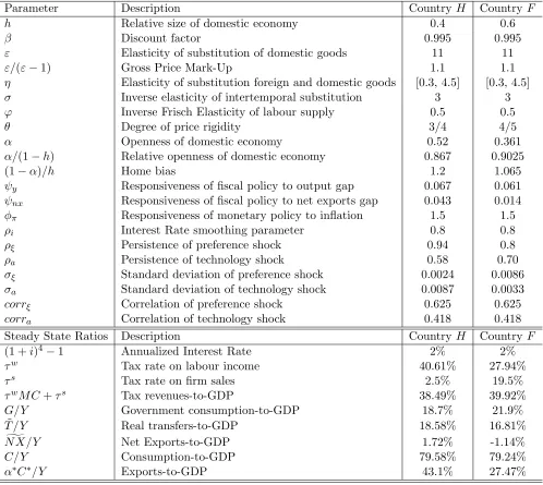
Parameter Description Country H CountryF

h Relative size of domestic economy 0.4 0.6

β Discount factor 0.995 0.995

ε Elasticity of substitution of domestic goods 11 11

ε/(ε−1) Gross Price Mark-Up 1.1 1.1

η Elasticity of substitution foreign and domestic goods [0.3, 4.5] [0.3, 4.5]

σ Inverse elasticity of intertemporal substitution 3 3

ϕ Inverse Frisch Elasticity of labour supply 0.5 0.5

θ Degree of price rigidity 3/4 4/5

α Openness of domestic economy 0.52 0.361

α/(1−h) Relative openness of domestic economy 0.867 0.9025

(1−α)/h Home bias 1.2 1.065

ψy Responsiveness of fiscal policy to output gap 0.067 0.061

ψnx Responsiveness of fiscal policy to net exports gap 0.043 0.014

φπ Responsiveness of monetary policy to inflation 1.5 1.5

ρi Interest Rate smoothing parameter 0.8 0.8

ρξ Persistence of preference shock 0.94 0.8

ρa Persistence of technology shock 0.58 0.70

σξ Standard deviation of preference shock 0.0024 0.0086

σa Standard deviation of technology shock 0.0087 0.0033

corrξ Correlation of preference shock 0.625 0.625

corra Correlation of technology shock 0.418 0.418

Steady State Ratios Description Country H CountryF

(1 +i)4−1 Annualized Interest Rate 2% 2%

τw _{Tax rate on labour income 40.61% 27.94%}

τs _{Tax rate on firm sales 2.5% 19.5%}

τw_{M C+τ}s _{Tax revenues-to-GDP 38.49% 39.92%}

G/Y Government consumption-to-GDP 18.7% 21.9%

˜

T /Y Real transfers-to-GDP 18.58% 16.81%

g

N X/Y Net Exports-to-GDP 1.72% -1.14%

C/Y Consumption-to-GDP 79.58% 79.24%

recent literature (SeeFerrero (2009) and Blanchard, Erceg and Lind´e(2015) for instance), but we also consider the case in which they are complements, as a robustness check for the effects of fiscal policy, as studied in Hjortsø(2016).

The calibration of the two countries mainly differs in the fiscal policy parameters. In particular, the government consumption-to-GDP ratios have been set respectively to 18.7% for country H and 21.9% for country F, according to the average of the last 9 years (source ECB-SDW). The marginal tax rates on labour income have been set respectively to 40.61% for country H and 27.94% for country F in accordance to the average in the last 9 years of the labour income tax wedges, excluding social security contributions made by the employer, for the median individual, as reported inOECD(2015). The marginal tax rate on firm sales has been set to 19.5% for country F according to the average VAT in the last 9 years for France, Italy, Spain and the Netherlands as reported in Eurostat, European-Commission et al. (2015), while it has been calibrated for country H to match the average ratio of net exports-to-GDP of 1.73% observed over the past 9 years for Germany13. Although the observed VAT rate for Germany is 19%, we set its marginal tax rate on firm sales to 2.5%, as if there were a production incentive, to correct for the fact that country H should have a greater productivity compared to country F, as Germany has a greater productivity than the Rest of the Euro Area. This calibration implies a steady state tax revenue-to-GDP ratio of respectively 38.49% for country H and 39.92% for country F, clearly in line with the data observed over the past decades for Germany (38.72%) and for France, Italy, Spain and The Netherlands (39.15%). Finally, the annualized steady state value of government debt-to-GDP in both countries is set to roughly 60% as stated in the Maastricht Treaty.

Since the two countries’ fiscal policy ratios have been calibrated according to the data, the transfers-to-GDP ratios have been set such that the government deficit is zero in steady state, which for country H reads:

˜

T Y = (τ

s_+τw_{M C)−} G

Y −

1

β −1

_˜

BG

Y (3.0.2)

Henceforth, the overall calibration of the fiscal sector implies a steady state ratio of transfers-to-GDP of respectively 18.58% for country H and 16.81% for country F, and a steady state ratio of current expenditure-to-GDP of respectively 37.28% for country H and 38.71% for country F. This calibration is broadly in line with the observed data over the last 10 years for the subsidies-to-GDP ratio (26.85% for Germany and 24.69% for the other countries) and the current expenditure (less interest)-to-GDP ratio (35.54% for Germany and 36.85% for the other countries).

In terms of model dynamics, the possible paths for government debt pose stability issues for the identification of a unique and stable solution of the model because, under wide circumstances, there might be an over-accumulation of debt and its dynamics might turn out explosive. We assume a real debt stabilization rule to achieve model stability, according to which in each period the nominal

13_{The average current account to GDP ratio observed over the past 9 years for Germany is roughly 6.36%. However,}

deficit is financed by tax rate movements. Indeed, to close the budget constraint, the government is assumed to rely on a combination of taxes on labor income and on firm sales. Specifically, γ in equation2.5.5indicates the share of the required change in total taxes that is allotted to the change in the labor income tax rate (1−γ is the share for the sales tax rate). In particular, with a few exceptions, the baseline calibration assumesγ = 0.5, which implies that the government balances the budget by increasing or decreasing equally the two tax rates with respect to steady state. Although the government debt level does not affect the equilibrium allocation between the two countries, once its steady state is assumed different from zero, it affects the dynamics of the model because of the interest rate paid on the nonzero stock of debt. Furthermore, this assumption is partially abandoned in the Full Fiscal Union scenario and it allows to show the additional stability gains from a greater fiscal capacity.

Although in the model a zero-deficit rule implies that the government budget must be kept con-stant by adjusting taxes, the feedback rule on government spending which reacts to output might trigger the tax ability to stabilize the economy. However, stability concerns are dissipated first, by having some degree of fiscal policy inertia, and second, by considering only rules which stabilize the output-gap or the net-exports gap. The autoregressive parameters for the fiscal rules have been estimated employing the time series for Germany, France, Italy and Spain for final consumption of the general government under the assumption of exogenous government consumption, following the same approach as for the technology shock (see below). The selection of the optimal fiscal policy parameters, instead, follows from the welfare analysis of the fiscal policy rules used in our model (see Section 5). As a measure of welfare, we consider the weighted average of the second order approximation of the utility of households in each country and the fiscal policy parameters have been selected to maximize the unconditional expectation of lifetime utility of the total popu-lation of households14 _{under the condition that they induce a locally unique rational expectations} equilibrium15.

Regarding the dynamic parametrization of the model, all exogenous shocks are assumed to follow a VAR(1) process that generally allows for both direct spillovers and second order correlation of the innovations. However, the structure has been restricted for both the technology shocks and the preference shocks to exclude direct spillovers.

With the exception of the preference shocks, whose dynamics have been calibrated following

Kollmann et al.(2014), the parameters characterizing the dynamics of the technology shocks have been estimated employing the time series for Germany, France, Italy and Spain of labour pro-ductivity per hours worked. All the series are chain-linked volumes re-based in 2010, seasonally

14_{Even if in the Pure Currency Union scenario the fiscal decisions are taken independently, we consider the results}

of the joint maximization of average aggregate welfare because it is in line with the results of a dynamic game between the two countries.

15_{Following Schmitt-Groh´e and Uribe(2007), we discretize the policy space by means of a grid search, because}

adjusted and filtered by means of a Hodrick-Prescott filter. The sample considered spans at quar-terly frequency from 2002 Q1 to 2015 Q3. Finally, despite a large debate on the high correlation between preference shocks in the Euro Area, there is no proper reference in the literature for its calibration. We decide to set this parameter according to the observed business cycle correlation (which is roughly 0.5) and we pick the value that maximizes the simulated correlation between output in the two countries (which is roughly 0.42)16_.

4

Numerical Simulations

We simulate the model numerically using Dynare17 (Adjemian et al.,2011), which takes a second-order approximation of the model, followingSchmitt-Groh´e and Uribe(2004), around its symmetric non-stochastic steady state with zero inflation and constant government debt. We compare the impulse response functions of the main variables to negative supply and demand shocks of one standard deviation, under a range of fiscal policy specifications, to study the stabilization properties of different coordination strategies and financing schemes.

In our simulations we analyze the impulse responses to a negative technology shock in country H or to a negative preference shock in country F. These two shocks account well for the dynamics in the Euro Area. A supply shock is more relevant in country H (calibrated on German data), which is the main producer and exporter of goods and services. On the other hand, country F (modeled as the Rest of the Euro Area), relies heavily on imports, hence a demand shock is crucial in driving its overall volatility.

4.1 Fiscal Policy Coordination

In the following graphs we simulate the model after a negative technology shock in country H and after a negative preference shock in country F, comparing the dynamics under the three different degrees of fiscal policy coordination – Pure Currency Union, Coordinated Currency Union and Full Fiscal Union – assumed in the paper. The financing scheme for these simulations is given by a balanced mix of the two tax rates, corresponding to the case γ = γ∗ = 0.5 18. The impulse responses are shown in Figure2 and Figure3, respectively.

After a negative technology shock in country H, marginal costs increase, bringing to an increase in prices and a decrease in output. Taxes increase to balance the government budget, which pushes prices and thus domestic inflation to rise, reinforcing the effect on prices of the increase in marginal costs. The consequent monetary policy tightening drives lower consumption in both countries, due to the assumption of complete markets. Since prices in country H are more flexible than those in

16_{The simulated values of the correlation of business cycles in our model, given our calibration, are always lower}

than the observed correlation. Therefore, we decide to select the correlation of preference shocks that maximizes the correlation of business cycles.

17_{All the equilibrium conditions of the model used for the simulations are shown in AppendixA.1.}

18_{Even if we show that the amplification of the shocks is increasing in γ, we prefer to use balanced financing}

Figure 2: Fiscal Policy Coordination - Technology Shock in Country H

Mix of Tax on Wage and on Sales ( . = 0.5) - Technology Shock in Country H

Quarterly values in % deviation from s.s. except Taxes and Interest Rate in p.p. difference from s.s.

0 10 20 -0.5

0

0.5 Total Taxes (H)

0 10 20 -0.4

-0.3 -0.2 -0.1 0

0.1 Gov. Cons. (H)

0 10 20 -0.6

-0.4 -0.2 0

0.2 GDP (H)

0 10 20 -0.06

-0.04 -0.02

0 Consumption (H)

0 10 20 -0.4

-0.2 0

0.2 Total Taxes (F)

0 10 20 -0.05

0 0.05

0.1 Gov. Cons. (F)

0 10 20 -0.1

0 0.1 0.2 0.3

0.4 GDP (F)

0 10 20 -0.06

-0.04 -0.02 0

0.02 Consumption (F)

0 10 20 -30

-20 -10 0

10 Net Exports (H)

0 10 20 -0.2

-0.15 -0.1 -0.05 0

0.05 Terms of Trade (H)

0 10 20 0

0.01 0.02

0.03 Interest Rate

Pure Currency Union Coordinated Currency Union Full Fiscal Union

country F, the terms of trade fall, inducing a deterioration in net exports for country H. Moreover, due to higher labor income taxes, domestic labour supply falls. The effect on labour supply and on net exports, in turn, amplifies the recession in country H and determines an expansion in country F, reinforced by the decrease in taxes and by the increase in government consumption.

A negative preference shock in country F, instead, decreases consumption and thus prices in country F, inducing higher labour supply and output. Country F can reduce taxes to balance the budget: as a consequence there is a further reduction of prices and inflation. The central bank reacts to lower overall inflation reducing the interest rate which, in turn, stimulates private consumption in country H. As observed for the technology shock, the terms of trade drop, in this case also due to the opposite dynamics of consumption, inducing net exports to fall, thus amplifying the recession in country H and the expansion in country F.

Figure 3: Fiscal Policy Coordination - Preference Shock in Country F

Mix of Tax on Wage and on Sales ( . = 0.5 ) - Preference Shock in Country F

Quarterly values in % deviation from s.s. except Taxes and Interest Rate in p.p. difference from s.s.

0 10 20 -0.4

-0.2 0 0.2

0.4 Total Taxes (H)

0 10 20 -0.4

-0.3 -0.2 -0.1 0

0.1 Gov. Cons. (H)

0 10 20 -0.6

-0.4 -0.2 0

0.2 GDP (H)

0 10 20 0

0.02 0.04 0.06

0.08 Consumption (H)

0 10 20 -1

-0.5 0

0.5 Total Taxes (F)

0 10 20 -0.05

0 0.05 0.1

0.15 Gov. Cons. (F)

0 10 20 0

0.2 0.4

0.6 GDP (F)

0 10 20 -0.2

-0.15 -0.1 -0.05 0

0.05 Consumption (F)

0 10 20 -20

-15 -10 -5 0

5 Net Exports (H)

0 10 20 -0.3

-0.2 -0.1 0

0.1 Terms of Trade (H)

0 10 20 -0.04

-0.03 -0.02 -0.01

0 Interest Rate

Pure Currency Union Coordinated Currency Union Full Fiscal Union

in the domestic output gap, caused by a negative technology shock in country H (Figure 2) or by a negative preference shock in country F (Figure 3). In order to guarantee a balanced budget, the tax rates vary in the same direction as government consumption. However, the movements in distortionary taxes offset the use of government consumption to stabilize output. As a result, consumption and prices are very volatile, and even output is sensibly more volatile compared to the other two fiscal policy scenarios.

volatile, so that international spillovers (net exports) are reduced and the economy (especially output) is more stable. Specifically, both a negative technology shock in country H and a negative preference shock in country F induce a deterioration in the terms of trade and a re-balancing of household consumption baskets. By stabilizing net exports, the terms of trade are consequently more stable, reducing the international substitution effect. As a result, the dynamics are much more amplified in the Pure Currency Union scenario and much less amplified in the Coordinated Currency Union scenario (dashed red line). By targeting the net exports gap, government consumption becomes procyclical instead of countercyclical. While the procyclicality induces more volatility, the need to balance the budget using distortionary taxation is able to lead to more stable dynamics compared to the countercyclical fiscal policy rule in the Pure Currency Union scenario. A similar finding can be obtained in a setup where debt is not constant. As shown in Coenen, Mohr and Straub (2008), tax-based consolidations could reduce the volatility of output, inflation and the terms of trade. Also according to Cardani, Menna and Tirelli(2018) the optimal policy for public debt consolidations, in contrast with empirical literature, calls for increases in taxes and inflation. The Full Fiscal Union scenario (dotted blue line) presents dynamics which are very close to those of the Coordinated Currency Union scenario, because in both cases government consumption targets the net exports gap. As highlighted above, there is a significant gain in terms of stabilization when the government targets the net exports gap, while if we also consolidate budget constraints we obtain very small improvements in terms of stabilization (the dashed red line and the dotted blue line follow very close paths). However, the joint movement in the tax rates makes the terms of trade more stable, reducing international spillovers and bringing government consumption to react less in the Full Fiscal Union scenario compared to the Coordinated Currency Union scenario. This produces more stable dynamics of output in both countries.

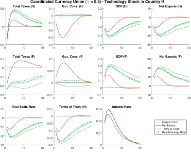
In order to check how our results depend on the common international target for fiscal policy coordination, we simulate the model using alternative common international targets, like the real exchange rate or the terms of trade19_{. In Figure 4 we compare the dynamics after a negative} technology shock in country H of four different targets for government consumption: domestic output in the Pure Currency Union scenario (dotted gray line), net exports (solid red line), the terms of trade (dashed blue line) and the real exchange rate (big dotted green line) under the Coordinated Currency Union scenario.

After a negative technology shock in country H, the terms of trade and the real exchange rate fall, bringing consequently to a fall in net exports and inducing country H to reduce government consumption, while country F increases it, with all fiscal policy targets except for output. Since net exports fall in country H, GDP falls in country H and rises in country F, bringing taxes to rise in country H and fall in country F to balance the government budget. The overall inflationary pressure determines a more aggressive monetary policy tightening compared to the case in which the common international target is net exports. The higher interest rate amplifies consumption

19_{The coefficients for the response of government consumption to either the real exchange rate or the terms of}

Figure 4: Targets For Coordination - Technology Shock in Country H

Coordinated Currency Union ( . = 0.5) - Technology Shock in Country H

Quarterly values in % deviation from s.s. except Taxes and Interest Rate in p.p. difference from s.s.

0 10 20 -0.5

0

0.5 Total Taxes (H)

0 10 20 -0.4

-0.3 -0.2 -0.1 0

0.1 Gov. Cons. (H)

0 10 20 -0.6

-0.4 -0.2 0

0.2 GDP (H)

0 10 20 -30

-20 -10 0

10 Net Exports (H)

0 10 20 -0.3

-0.2 -0.1 0

0.1 Total Taxes (F)

0 10 20 -0.05

0 0.05

0.1 Gov. Cons. (F)

0 10 20 -0.1

0 0.1 0.2 0.3

0.4 GDP (F)

0 10 20 -10

0 10 20

30 Net Exports (F)

0 10 20 -0.03

-0.02 -0.01 0

0.01 Real Exch. Rate

0 10 20 -0.2

-0.15 -0.1 -0.05 0

0.05 Terms of Trade (H)

0 10 20 0

0.01 0.02

0.03 Interest Rate

Output (PCU) Net Exports Terms of Trade Real Exchange Rate

and thus output dynamics in both countries, making the stabilization of international variables less effective. Furthermore, total taxes in country F follow the opposite path of GDP with all targets except for net exports. This reversal of the dynamics of total taxes with target net exports (solid red line) with respect to other targets is given by the much smaller increase in the tax base (GDP) and much greater increase in the response of government consumption, which brings taxes to increase rather than decrease, stabilizing relative prices and thus net exports more than with other targets.

future. On the other hand,Forni and Pisani(2018) assesses the macroeconomic effects of sovereign restructuring in a small open economy belonging to a monetary union, showing that restructuring can imply persistent and large reductions in output. A natural question then could be to assess how the desirability of reducing international imbalances holds when debt is not constant over time. In a similar setup, Cole et al.(2016) considers the case in which one country belonging to a Currency Union needs to deleverage. It finds that when countries coordinate on an international target (such as net exports), this reduces overall volatility, in particular that of output and the terms of trade.

4.2 Alternative Financing Schemes

Here we analyze the qualitative implications of the model, by varying the percentage financed by the tax rate on labour income with respect to the tax rate on firm sales. More in detail, we simulate the model under three combinations ofτs _{and τ}w_:

• γ = 0.2, financed roughly 20% by varying the tax rate on labour income and 80% by varying the tax rate on firm sales.

• γ = 0.5, financed roughly by varying equally the two tax rates. This can be considered as the baseline financing scheme, followed in all other simulations.

• γ = 0.8, financed roughly 80% by varying the tax rate on labour income and 20% by varying the tax rate on firm sales.

We also compare the outcomes of financing fiscal policy with lump-sum taxes, which do not produce distortions in the economy. Figures 5 and 6 show the impulse responses with different financing schemes to a negative technology shock in country H in the Pure Currency Union scenario and in the Full Fiscal Union scenario, respectively20_.

In the Pure Currency Union scenario (Figure 5), when distortionary taxation is used by the governments, the dynamics are much more volatile than in the case in which lump-sum taxes finance government expenditure. As an example, if we compare the financing scheme in which the burden is shared equally by the two tax rates (solid red line) with the case in which non-distortionary taxation is used (dotted gray line), we can observe that both interest rate and output are much more stabilized with the latter financing scheme. Furthermore, the amplification of the shocks is increasing exponentially inγ, with the most amplified dynamics given by the massive use of the tax rate on labour income (γ = 0.8, dashed blue line) to finance fiscal policy. When governments use distortionary taxation, the most stable dynamics are given by varying mainly the tax rate on firm sales (γ = 0.2, dashed-dotted green line), while varying equally the two tax rates (γ = 0.5, solid red line) creates a little more distortion compared toγ = 0.2 and much less distortion compared to

γ = 0.8. Therefore these results point out to the fact that taxes on labour income are much more distortionary than taxes on firm sales.