Generating Spatial Descriptions for
Cross-modal References
P e t e r
Wazinski
SFB 314, Department of Computer Science
University of Saarbrficken
D-6600 Saarbrficken, Germany
email: [email protected]
A b s t r a c t
We present a localisation component that sup- ports the generation of cross-modal deictic ex- pressions in the knowledge-based presentation system WIP. We deal with relative localisations (e.g., "The object to the left, of object X."), absolute localisations (e.g., "The object in the upl)er left part of the l)icture.") and corner lo- calisations (e.g., "The object in the lower right corner of the l)icture"). In addition, we distin- guish two localisation granularities, one less de- tailed (e.g., "the object to the left. of object X.") and one more detailed (e.g., "the object above and to the left. of object X."). We consider cor- ner localisations to be similar to absolute local- isations and in turn absolute localisations to be specialisations of relative localisations. This al- lows us to compute all three localisation types with one generic localisation procedure. As elementary localisations are derived from pre- viously computed composite localisations, we can cope with both localisation granularities in a computationally efficient way. Based on these l)rimary localisation l)rocedures, we dis- cuss how objects can be localised among several other objects. Finally we introduce group local- isations (e.g., "The object to left, of the group of or, her objects.") and show how to deal with thern.
1 I n t r o d u c t i o n
The increasing a m o u n t of information to be communi- cated to users of complex technical systems nowadays makes it necessary to find new ways to present infor- mation. Neither the variety of all possible l)resentation situations can be anticipated nor it is fiLrther adequate to present the required information in a single communi- cation mode, such as either text or graphics. Therefore, the automatic generation of nmltimodal presentations tailored to the individual user has become necessary. Current research projects in artificial intelligence like SAGE ([Roth et al., 1990]), F N / A N D D ([Marks and Reiter, 1990]), C O M E T ([Feiner and MeKeown, 1990])
and W I P ([Wahlster el al., 1991a]) reflect the growing interest in this topic.
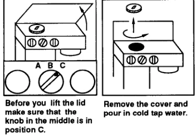
For the knowledge-based presentation system WIP, the task is the generation of a multimodal document ac- cording to the formal description of the communicative intent of the planned presentation and a set of generation parameters. T h e current scenario for W I P is the gener- ation of instructions for using an espresso-machine. A typical fragment of an instruction manual for an espresso machine is shown in figure 1.
b
I
A B C
© ® ©
Before you lift the lid make sure that the knob in the middle is in position C.\ o
\ ® ¢ ®
Remove the cover and pour in cold tap water.
Figure 1: Fragment from an instruction manual
Cross-modal deictic expressions, e.g., "the lid" or "the knob in the middle," help to establish the coreferentiality between the entities mentioned in the text and shown in the picture as well ([Wahlster et al., 1991b]). T h e use o! spatial relationships such as "the knob in the middle" simplifies the generation of referring expressions that have to identify a particular object in a picture. Ob- viously these spatial relationships cannot be computed in advance because they depend on the projection para- meters for the picture, e.g., the viewpoint, which in turn themselves depend on the communicative intent of the document to be planned 1.
The localisation component described in this paper was developed in order to support the generation ot cross-modal deietic referring expressions. All procedures are fully implemented and were recently integrated intc the first W I P prototype. T h e y are coded in C o m m o r
[image:1.612.376.568.336.469.2]Lisp and run under Genera 8.0 on a Maclvory. A testbed called LOC-SYS was also developed: it allows the con- venient generation and manipulation of rectangle scenes like the examples given in this paper.
Before we describe the methods which underlie the various localisation procedures, in the following section we present our views about localisation phenomena and introduce the terminology used in the rest of this paper.
2
Object Localisation
A lot of work has been done on 'object localisation' and its linguistic complelnent, 'spatial l)repositions'. Wunderlich/Herweg ([Wunderlich, 1982], [Wunderlich and Herweg, forthcoming]) and Herskovits ([Herskovits, 1985]) provide linguistic approaches to the semantics of spatial prepositions. NL-systems like NAOS ([Neumann and Novak, 1986]), HAM-RPM ([Hahn el al., 1980]), SWYSS ([HuBmann and Schefe, 1984]) and C'ITYTOUR ([Andr~ et al., 1985],[Andr~ et al., 1986]) address var- ious issues regarding computational aspects. Schirra ([Schirra, to appear 1992]) and Habel/Pribbenow ([Ha- l)el and Pribbenow, 1988],[Pribbenow, 1990]) also incor- porate relevant work from cognitive psychology.
In our approach, we concentrate on the requirements for localising objects ill pictures. We assume that the user can see the picture containing the objects to be localised and we do not deal with the problem of an- ticipating possibly wrong visualisations of the user in the case he/she cannot see the picture. We do not deal with possible intrinsic orientations of depicted objects (c.f. [Retz-Schlnidt, 1988]) and assume the deictic refer- ence frame of a common viewer (c.f. figure 5). Together with every localisation, we compute a so-called applica- bility degree from the intervall [0..1]. The applicability degree is not only used to generate linguistic hedges (c.f. [Lakoff, 1972]) as in SWYSS or C I T Y T O U R , but also for selecting the 'best' localisation from a set of alter- natives. The localisations computed on our system are two-dimensional localisations in the sense that they are based on the 2D-projection of a picture aim not on its possible 3D-representation. In the rest of this section we will describe the localisation phenomena we take into account and introduce our terminology.
2.1 R e l a t i v e a n d a b s o l u t e l o e a l i s a t i o n s
The objects shown in part A of figure 2 can be localised as follows:
B
%% jS S I I
.
I
A° R
Figure 2: Localising objects in a picture
(1) "Object A is on the right side of the picture."
(2) "Object B is ill the lower part of the picture." (3) "Object A is to the right of Object B." (4) "Object B is below Object A."
Sentences (1) and (2) are considered to contain a b - s o l u t e localisations: an object is localised by stating its absolute position in the picture. Sentences (3) and (4) are examples of r e l a t i v e l o c a l i s a t i o n s : an object is localised by stating its position relative to another ob- ject. The object to be located will be called the p r i m a r y o b j e c t (LO for short). T h e object that serves as refer- ence for locating the primary object is called r e f e r e n c e o b j e c t ( R E F O for short).
How can we explain the similarity between absolute and relative localisations, between "on the right side of the picture" and "to the right of Object B"? Our hy- 1)othesis is:
Absoh'lte localisations are specialisations of relative localisations in the sense that for ab- solute localisations the center of the picture functions as an implicit reference object.
Part B of figure 2 shows how the absolute localisation of part A can be explained as a relative localisation by assuming a circle-shaped center: "Object A is on the right side of the picure." is equivalent to "Object A is to the right of the center of the picture."
2.2 E l e m e n t a r y a n d c o m p o s i t e localisations
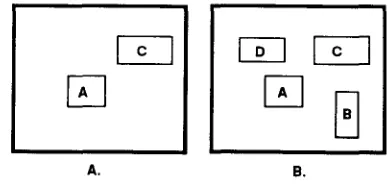
Whereas the unambiguous localisations of the objects in figure 2 could be achieved by naming either the horizon- tal ("on the right side", "to the right of") or vertical relation ("in the lower part", "below"), figure 3 shows a situation in which it is necessary to give both the hori- zontal and vertical position of the object with respect to the reference object:
5-1
yz-q
D[q
A, B,
Figure 3: Elementary and composite localisations
Ill part A of figure 3, it is sufficient to describe object C as the object "to the right of" or "above" object A. But in part B, both descriptions would be ambiguous, because "to the right of" or "above" could refer to object D or B respectively. The only possibility to localise C unambiguously is to describe it as being "above and to the right" of A.
Localisations where either the horizontal or vertical relation is given will be called e l e m e n t a r y l o c a l i s a - t i o n s . If both relations are stated together, we will call it a c o m p o s i t e localisation.
[image:2.612.341.535.436.529.2] [image:2.612.65.278.578.696.2](;omposite localisations cannot always he applied, e.g., in figure 2 object B cannot be localised as "the object in the lower left p a r t of the picture." Criteria for the applicability of composite localisations will not he ex- alnined further in this paper as this would lead to more complex questions, e.g., whether an object can be lo- calised at all. A detailed discussion of these prohlems is given in [Wazinski,
1991].
2.3 T h e c o n s t r u c t i o n o f t h e h o r i z o n t a l a n d v e r t i c a l r e f e r e n c e f i ' a l n e
One i m p o r t a n t feature of the localisation l)rocedures is the division of the horizontal and vertical reference frame into three parts. T h e reason for this are 'center'- localisations as shown in figure 4:
Figure 4: Center localisations
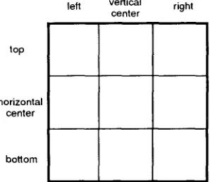
In all pictures, object A can be localised as tile object "in the center of the 1)icture." In order to integrate this observation with the elementary vs. composite distinc- tion we divided the horizontal and vertical dimension into three parts: ' t o p ' , 'horizontal center' and ' b o t t o m ' and 'left', 'vertical center' and ' t o p ' respectively (c.f. fig- ure 5). Under these conditions the 'center'-localisation in the left part of figure 4 can be analysed as a com- posite ('vertical center','horizontal center')-localisation. For the picture in the middle it is an elementary 'verti- cal center'-localisation and for the right one an elemen- tary 'horizontal center'-localisation. When transforming these different localisations into a surface string they all become the same: "in the center of the picture."
left vertical right center
top
horizontal center
"to the right of A" by assuming t h a t the ' c e n t e r ' - p a r t of a composite localisation is a special p a r t of a composite localisation t h a t does not a p p e a r at the linguistic level.
Yl
YlV
Figure 6: Center localisations and relative localisations
2.4 C o r n e r L o e a l i s a t i o n s
An additional localisation type t h a t can be used to lo- calise objects in pictures is the c o r n e r l o c a l i s a t i o n : if an object is placed in one of the four corner regions of the picture it can be localised as, e.g., "the object in the
left u p p e r c o r n e r of the picture."
Tile difference between absolute composite localisa- tions and corner localisations is illustrated in figure 7: While object B can be localised as being "in the lower right corner of the picture" it is not possible to use a corner localisation for A. In t h a t case, only "in the left upper part of the picture" could be used. Therefore, we consider corner localisations to be more precise t h a n ab- solute composite localisations, i.e., the applicability of a corner localisation implies the applicability of the cor- responding absolute composite localisation but not vice versa.
A
Figure 7: Corner localisations vs. absolute composite localisations
bottom
Figure 5: Horizontal and vertical reference frame
Figure 6 shows that it, is also useful to adopt the this partition scheme for relative localisations: B would usually be described as the object "to the right of A" and C as the object "above and to the right of A." With respect to tile partition scheme a ('right', ' t o p ' ) - localisation can be applied to C and a ('right', 'horizontal center')-localisation to B, T h e former matches exactly with the surface string. T h e latter can be matched with
3
B a s i c L o c a l i s a t i o n P r o c e d u r e s
[image:3.612.412.519.106.200.2] [image:3.612.93.325.228.322.2] [image:3.612.412.525.431.542.2] [image:3.612.138.287.488.617.2]3.1 A b s o l u t e l o e a l i s a t i o n s
We a p p r o x i m a t e the center of the picture with a rect- angle whose horizontal and vertical extension is one third of the horizontal and vertical extension of the picture. Figure 8 shows the construction of the horizontal and vertical reference system according to the rectangular center region.
vertical right lell center
N
top
. . . ... .:.:.;,:,:,:.:.:.:.:.:.:.:.~ t :.:.:.:.:.:.:.:.:.:.:.:.:1
horizontal ll~|~iti:
center ::::::::::::::::::::::::::: :.:.:.
boHom
For object LO in f g u r e 9, the above definition yields the following results:
Ac((left, top), LO) = 1/12, A¢((x-center, top), LO) = 1/6, A~((left, y-center), LO) = 1/4, Ac((X-center, y-center), LO) = 1/2.
For all other 1 C CLOC we have A~(l, LO) = 0 because
f(P) = f(Po) = O.
left vertical center right
top 1 / 3
v4 ::Ni ::iii:i:---.-':!
hor, onta,
"::iiii Nii
center
Figure 8: Tile construction of tile horizontal and vertical reference system
Before describing the evaluation function for cornpos- ite localisations, we give a few definitions:
• T h e horizontal reference system is abbreviated by XLOC = {left, x-center, right}, the vertical one by
Y L O C ---- {top, y-center, b o t t o m } . Composite locali-
sations are denoted by CLOC = XLOC ×YLOC. Both
reference systems together are described with ULOC = XLOCI.JYLOC.
• T h e constant C E N T E R denotes the center rectangle of a given picture.
• POLY denotes the set of all polygons that can ap- pear in a picture. For given polygons P1 and P2 tile associative and c o m m u t a t i v e operator N, ("1 : POLY X POLY ~ POLY computes the in- tersection polygon. The e m p t y polygon is denoted by P0. T h e following holds: VP E POLY : P$ 71 P =
p n D ~ = P ~ .
• The fimction P R (Partial Rectangle), PR : CLOC x POLY ~ P O L Y , computes the rectangle correspond-
ing to a given composite localisation and the rec- tangle partition of the picture induced by a given polygon. For example PR((left,top), ( : E N T E R ) computes the upper left rectangle according to the partition scheme shown in figure 8.
• !R denotes the set of the real numbers. Given a polygon P, the fimction f, f : POLY ~ N computes the area of a polygon. It is f(P~) = O.
T h e applicability degree of a composite localisation evaluates how good the position of the object in ques- tion is described by t h a t particular localisation. We de- fine the applicability degree as the portion of the area of the object that lies in the rectangle of the picture that corresponds to the composite localisation and the rec- tangle partition of that picture. Thus we can define A~ as follows:
Ac : CLOC X POLY ~ ,~
A~(I, LO) = f ( p )
f ( L O )
with p = PR(I, C E N T E R ) Cl LO
bosom
Figure 9: C o m p u t i n g absolute localisations
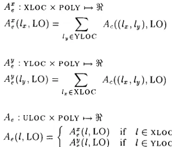
For elementary localisations we adopted an analogous definition: the applicability degree Ae of an elementary localisation is determined by the portion of the area of the object that lies in the corresponding row or column of the picture. As already mentioned at the beginning of this section we can write A~ in terms of A~ :
A~ : XLOC :x: POLY ~
A~(l,:, LO) : Z A~((l=, ly), LO)
l v E Y L O C
Ae y : YLOC × POLY
A~e(ly, LO) = ~ A~((l~:, ly), LO)
I=EXLOC
Ae : ULOC X POLY ~
,fi ,'
A~ and A~ c o m p u t e tile applicability for the horizon- tal and vertical dimension by s u m m i n g up the applicabil- ity degrees of the corresponding composite localisations. They are combined ill A¢ order to have a function t h a t is defined oll both dimensions, i.e., ULOC.
With respect to figure 9 we get:
A~(top, LO) = A¢((left, top), LO) + A¢((x- center, top), LO) = 1/4,
A~(y-center, LO) = A~((left, y-center), LO) + A¢((x-center, y-center), LO) = 3/4,
A~(left, LO) = A¢((left, top), LO) + Ac((left, y-center), LO) : 1/:3 aim
[image:4.612.62.294.153.265.2] [image:4.612.356.532.411.561.2]As argued in l)aragraph 2.4 corner localisations are similar to composite ( ' l e f t ' / ' r i g h t ' , ' t o p ' / ' b o t t o r n ' ) - localisations, but less general. This property can be modelled by corner regions that are smaller than tim corner regions for absolute localisations. In turn, these corner regions correspond to a larger center as shown in figure 10. Thus we can compute corner localisations just by changing the size of the center.
F
y
Figure 10: Tim relation between corner and center re- gions
Instead of
1/3
as for absolute localisations we take 4/5 of the horizontal and vertical extension of the picture for the extended center.3.2
R e l a t i v e l o c a l i s a t i o n sThe localisation procedure for relative localisations is similar to the one for absolute localisations. One ma- jor difference is that now the construction of the hori- zonta.l and vertical reference frame is done with respect to a given reference object and not to the implicit as- sumed center of the picture (c.f. figure 11). The second difference concerns the computation of the applicability degree: for relative localisations, not only the portion of an area is taken into account, but also the distance between the primary object and the reference object.
vertical
left center right
top
horizontal
center
bottom
Figure 11: The construction of the reference frame for relative localisations
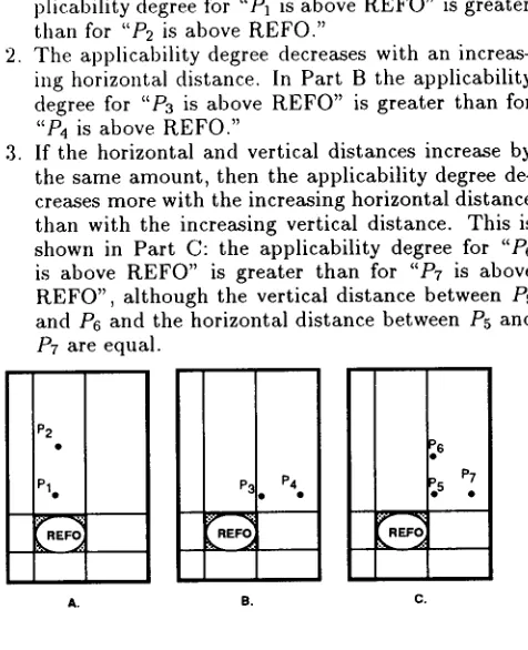
The basic idea for the evaluation of the distance be- tween primary object and reference object is adopted from the C,1TYTOUR system: first we compute the cen- ter of gravity for the primary object. Then we determine its coordinates with respect to the reference system es- tablished by the reference object. Finally we use these coordinates for the c o m p u t a t i o n of the applicability de- gree. Figure 12 illustrates the various factors that affect the applicability of an 'above'-localisation:
1. The applicability degree decreases with an increas- ing vertical distance. In Part A of figure 12 the ap-
2.
.
plicability degree for "P1 is above R E F O " is greater than for "P2 is above REFO."
The applicability degree decreases with an increas- ing horizontal distance. In Part B the applicability degree for "P3 is above R E F O " is greater than for "P4 is above REFO."
If the horizontal and vertical distances increase by the same amount, then the applicability degree de- creases more with the increasing horizontal distance than with the increasing vertical distance. This is shown in Part C: the applicability degree for "P6 is above R E F O " is greater than for "P7 is above R E F O " , although the vertical distance between P5 and P6 and the horizontal distance between P5 and /°7 are equal.
P2
• P.6
P1 e P3 P4 pe 5 P7
A B. C
Figure 12: Evaluating tile distance of a point Let eval denote the function that evaluates the dis- tance between a point and a rectangle according to the criteria mentioned above. Let further POINT denote the set of all points within a picture and RECT C POLY the set of all rectangular polygons. Then the signature oi
eval can be written as2:
eval : CLOC × P O I N T × R E C T ~ ~}~
Now we are almost able to define the function Ac, which computes the applicability degree of a composite lo- calisation. Let C G , C G : P O L Y ~ P O I N T , compute
the center of gravity for a polygon and let further SR,
S R : P O L Y ~ R E C T , compute the smallest surrounding
rectangle for a polygon. Then the applicability degree Ac of a composite localisation can be defined as:
A c : C L O C × P O L Y X P O L Y ~ {}~
Ac( l, LO, REFO) = w eval( l, CG(p), S R ( R E F O ) ) with p = PR(I, R E F O ) fq LO
f(P)
W - - -
-f ( L O )
[image:5.612.354.592.65.358.2] [image:5.612.86.332.153.249.2] [image:5.612.95.327.459.576.2]p is tile part of the primary object that lies in the rectangle corresponding to the composite localisation I. The factor w weighs the result of eval according to the portion of the area of the primary object that lies in the rectangle corresponding to I.
Now the definition of Ae, the applicability degree for an elementary localisation, can be given in terms of A~ again:
A~ : X L O C × P O L Y × P O L Y ~
A~(l~, LO, REFO) = ~ A¢((b:, Iv), LO, REFO)
I u E Y L O C
A~
: Y L O C × P O L Y × P O L Y ~A~(l v LO, REFO) = ~ A~((I~, Iv), LO, REFO)
I : : E X L O C
Ae
: U L O C X P O L Y × P O L Y ~Ae(I, LO, R E F O ) = I A~(I, LO, R E F O ) if l E XLOC
• A~(l, LO, REFO) if l E YLOC
This means that the applicability degree Ae for a pri- mary object LO is the sum of the coml)osite localisa- tions for tlle corresponding row or colunm of tile refer-
e n c e fr anle.
For figure 1:3 we get, the following results: A~((x-center, top), LO, REFO)
- 5 - l eval((x-center, top), P1, SR(REFO)
_ _ 1
- 5 " 0 " 7 = 0 " 2 3
A~((right, top), LO, REFO)
_ 2 eval((right, top), P2, S R ( R E F O ) - 5
2
= 5 * 0.65 = 0.43
A¢(l, LO, REFO)
= 0 as for all other I E CLOC: : w -- - - f ( P ) -- 0
f ( L O ) Ae(top, LO, REFO)
= Ac((x-center, top), LO, R E F O ) + A~((right, top), LO, REFO) = 0.66
A~(right, LO, REFO)
= A~((right, top), LO, REFO) = 0.43
Ae(x-center, LO, REFO)
= A¢((x-center, top), LO, REFO) = 0.23
4
A generic localisation p r o c e d u r e for
absolute
a n d r e l a t i v e l o c a l i s a t i o n s The similarities between the localisation procedures dis- cussed in the previous section allow us to design one generic localisation procedure that can be specialised to a procedure for absolute, relative or corner localisations. Given the primary object, LO and the reference object REFO the first step is to determine the 3 x 3 matrix M n, which contains the intersection polygons of LO and the partial rectangles in the picture with respect to REFO. For relative localisations, REFO varies, for absolute lo- calisations and corner localisations the parameter is set to either the normal or the extended center area (c.f. section 3.1). Thus, for x E XLOC, y E YLOC we computeM ~ v = P R ( ( x , y), REFO) M LO
P2
Pl[-LO •
]113 2/3
REFO
j.,.
Figure 13: Computing relative localisations
The second step is the c o m p u t a t i o n of the evaluation matrix M A, which contains the applicability degrees of the composite localisations. T h e c o m p u t a t i o n requires a fimction E, E : P O L Y × P O L Y × P O L Y ~ ~ . E corresponds
exactly to the flmction Ae for absolute and relative local- isations in section 3.1 and 3.2. The only difference results from tile previous computation of Mn: tile subexpres- sion p = P R ( ( x , y), REFO) M LO is factored from A¢ and therefore computed only once.
MAu
= E(M2,u, LO, REFO)The third step is the c o m p u t a t i o n of the elementary lo- calisations. T h e vector )~ contains the evaluations of the horizontal localisations and ]7 the ones for the vertical localisations:
y E Y L O C
x E X L O C
This means that we have -~t = Ae(l) for l E XLOC and
= A~(l) for l E YLOC.
Finally, we can determine the best composite and el- ementary localisation and their applicability degrees by computing the m a x i m u m value of M A and X or )7 re- spectively.
For figure 13 we get
0 0.23 0.43 )
M A = 0 0 0 ,
0 0 0
~g = (0 0.2:3 o.43) and ~ = (0.66 0 0). The best compos- ite localisation is "(right, top)" with applicability degree 0.4:3. The best elementary localisation is "top" with ap- plicability degree 0.66.
5
Localising o b j e c t s in a c o m p l e x scene
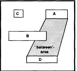
[image:6.612.349.481.63.192.2]In order to reduce the search space for REFO candi- dates, f r s t a kind of 'between'-test is applied to the set of possible reference objects. T h e idea behind this test is that an exclusion procedure based on simple geomet- ric overlapping tests can be performed more efficiently than a comparison of applicability degrees that have to be computed by the rather complex localisation proce- dures. An example is given in figure 14: When searching for a suitable reference object for object A in figure 14, object D would be ruled out because object B is found in the ' b e t w e e n ' - a r e a of A and D.
/Jiiiiiiiiiiiiiiiiiiiiiiiiiii "
l
I
o
I
Figure 14: Search space reduction for complex object configurations
The deterinination of the best reference object raises the problem of ambiguity. Not only is the applicability degree of a localisation i m p o r t a n t , but also whether the use of the reference object would result in an ambiguous localisation. In t h a t case, a different reference object has to be chosen. If all possible localisations are a m - biguous, then the particular object cannot be loealised at. all. E.g., in Part A of figure 15 object D could be localised as being either "above A" or "to the right of (:." But the first localisation is ambiguous because both, C and D, are "above A."
A. B. C.
Figure 15: Ambiguous reference objects
With respect to elementary and composite localisa- tions we distinguish three cases of ambiguity:
1. In Part A of figure 15, the localisation of object (I or D would be ambiguous with respect to A because for both objects the composite localisations, (x-center, top), are equal.
2. In Part B a composite localisation cannot be applied to object D (neither "D is above and to the right of A" nor "D is i m m e d i a t e l y above A" are adequate) and its elementary localisation, ' t o p ' , is part of the composite localisation, (x-center, top), of object C. 3. In Part C a composite localisation can be applied
neither to C nor to D and their elementary locali- sations, ' t o p ' , are equal.
6
Localising Groups of Objects
Control knobs and switches are often grouped together in a control panel in order to provide for easier operation of technical devices. Moreover spatially adjacent objects can also be grouped as one perceptual unit according to the 'law of the good gestalt' in G e s t a l t psychology ([Murch and Woodworth, 1978]). T h u s the possibility to generate loealisations with respect to a given group structure is neccessary for the "naturalness" of a local- isation. Besides this, group localisations are also useful if the objects in the i m m e d i a t e neighbourhood of the p r i m a r y object have exactly the s a m e properties (c.f. [Wahlster el al., 1978]). In this case, the p r i m a r y ob- ject can be localised with respect to its group and has not to be localised with respect to the whole scene, which could have resulted in an a m b i g u o u s localisation.
For our localisation procedures this means t h a t groups can function as a reference object as well as a p r i m a r y object.. In addition, objects can be localised absolutely with respect to the group they are contained in. In figure 16 object B would be localised as the object "to the right of the triangles." Vice versa we can say "The triangles to the left of object B" and we can localise object A as being "the upper left of the triangles t h a t are to the left of B."
Figure 16: G r o u p localisations
T h e last e x a m p l e also illustrates the hierarchical char- acter of group localisations: An object can be localisec absolutely within a group. T h i s group might be localisec again within a surrounding group or - - if there is non( - - this group can be localised relatively with respect t( another (group of) object(s).
T h e algorithm for group localisations cannot detecl group hierarchies. Instead it expects a tree representa- tion of tile group hierarchy as an input. T h e o u t p u t con sists of two parts: According to the depth of the grout tree the algorithm computes a chain of absolute locali sations. In addition the o u t e r m o s t surrounding group o the p r i m a r y object is localised relatively to an optiona (group of) reference object(s).
7
Conclusions
[image:7.612.146.279.188.311.2] [image:7.612.413.530.375.482.2] [image:7.612.98.316.478.567.2]for elementary localisations in terms of the evaluation fimctions for the corresponding composite localisations, we have been able to design one procedure that handles all three locMisation types and both localisation granu- larities efficiently. Furthermore, we have given a solution to the problem of localising an object within a complex configuration on the basis of this localisation procedure. Finally, we have shown how our system deals with group localisations.
R e f e r e n c e s
[Andr(~ el al., 1985] E. Andre, G. Bosch, G. Herzog, and T. Rist. CITYTOUR - Ein natiirlichsl)rachliches Anfragesystem zur Evahfierung r~umlicher Pr~posi- tionen. AbschlufJbericht des Fortgeschrittenenprak- tikums, Department of Computer Science, University of Saarbriicken, 1985.
[Andr~ el al., 1986] E. Andre, G. Bosch, G. Herzog, and T. Rist. Characterising Trajectories of Moving Ob- jects using Natural Language Path Descriptions. In
Proc. of the 7th ECAI, pages 1-8, 1986.
[Feiner and McKeown, 1990] S. K. Feiner and K. R. McKeown. Coordinating Text and Graphics in Expla- nation Generation. In Proc. 8th AAAI, pages 442-449,
1990.
[Habel and Pribl)enow, 1988]
C. Habel and S. Pribbenow. Gebietskonstituierende Prozesse. LILOG-Report 18, IBM Germany, 1988. [Hahn el al., 1980] W. v. Hahn, W: Hoeppner, A. Jame-
son, and W. Wahlster. The Anatomy of the Natural Language Dialogue System HAM-RPM. In L. Bole, editor, Natural Language Based Computer Systems,
pages 119-254. Miinchen: Hanser, 1980.
[Herskovits, 1985] A. Herskovits. Semantics and Prag- rnatics of Locative Expressions. Cognitive Science,
9:341-378, 1985.
[Hut3mann and Schefe, 1984] M. Huflmann and P. Sche- fe. The Design of SWYSS, a Dialogue System for Scene Analysis. In L. Bole, editor, Natural Language Communication with Pictorial Information Process-
ing. Miinchen: Hanser McMillan, 1984.
[Lakoff, 1972] G. Lakoff. Hedges: A Study in Meaning Criteria and the Logic of Fuzzy Concepts. In J.N. Levi and G.C. Phares, editors, Papers fi'om the 8th regional Meeting of the Chicago Linguistics Society,
pages 183-228. University of Chicago, Chicago, IL, 1972.
[Marks and Reiter, 1990] 3. Marks and E. Reiter. Avoiding Unwanted Conversational hnplicatures in Text and Graphics. In Proc. 8th AAAI, pages 450- 455, 1990.
[Murch and Woodworth, 1978] G.M. Murch and G.L. Woodworth. Wahrnehmung. Stuttgart: Kohlhamlner, 1978.
[Neulnann and Novak, 1986] B. Neurnann and H.-J. No- vak. NAOS: Ein System zur natiirlichsprachlichen Beschreibung zeitveriinderlicher Szenen. Informatik
Forschuuy und Eutwickluug, pages 83-92, 1986.
[Pribbenow, 1990J s. Pribbenow. Interaktion yon propo-
sitionalen und bildhaften ReprS.sentationen. In C. Ha- be/ and C. Freksa, editors, Repriisenlation und Ver-
arbeitun9 rdmlichen Wissens, pages 156-174. Berlin:
Springer, 1990.
[Retz-Schmidt, 1988] G. Retz-Schmidt. Various Views on Spatial Prepositions. A I Magazine, 9(2):95-105, 1988.
[Roth et al., 1990] S. Roth, a. Mattis, and X. Mesnard. Graphics and Natural Language as Components of Automatic Explanation. In d. W. Sullivan and S. W. Tyler, editors, Intelligent User Interfaces, pages 207- 239. Reading, MA: Addison Wesley, 1990.
[Schirra, to appear 1992] J. Schirra. A Contribution to the Reference Semantics of Spatial Prepositions: The Visualization Problem and its Solution in VITRA. In
Proceedings of the IAI Workshop "On the Semantics
of Prepositions in Natural Language Processing. Mou-
toll, de Gruyter, to appear 1992. Also available as Technical Report 75, SFB 314, Department of Com- puter Science, University of Saarbriicken.
[Wahlster et al., 1978] W. Wahlster, A. Jameson, and W. Hoeppner. Glancing, Referring and Explaining in the Dialougue System HAM-RPM. American Journal
of Computer Linguistics, Microfiche 77, pages 53-67,
1978.
[Wahlster et al., 1991a]
W. Wahlster, E. Andr4, S. Bandyopadhyay, W. Graf, and T. Rist. WIP: The Coordinated Generation of Multimodal Presentations from a Common Represen- tation. In O. Stock, J. Slack, and A. Ortony, editors,
Computational Theories of Communication and their
Applications. Berlin: Springer, 1991.
[Wahlster et al., 1991b] W. Wahlster, E. Andr4, W. Graf, and T. Rist. Designing Illustrated Text: How Language Production is Influenced by Text and Graphics. In Proc. 5th Conf. of the European Chap- ter of the Association for Computational Linguistics
(EACL), pages 8-14, 1991.
[Wazinski, 1991] P. Wazinski. Objektlokalisation in gra- phischen Darstellungen. Master's thesis, Universitgt Koblenz-Landau, Abt. Koblenz/DFKI Saarbriicken, 1991.
[Wunderlich and Herweg, forthcoming] D. Wunderlich and M. Herweg. Lokale und Direktionale. In A. v. Stechow and D. Wunderlich, editors, Handbuch der
Semantik. Kgnigstein Ts.: Athengum Verlag, forth-
coming.
[Wunderlich, 1982] D. Wunderlieh. Sprache und Raum.