Contextual Spelling Correction Using Latent Semantic Analysis

(1)

C o n t e x t u a l Spelling Correction Using Latent Semantic Analysis

M i c h a e l P . J o n e s a n d J a m e s H . M a r t i n

D e p t . o f C o m p u t e r S c i e n c e a n d I n s t i t u t e o f C o g n i t i v e S c i e n c e U n i v e r s i t y o f C o l o r a d o

B o u l d e r , C O 8 0 3 0 9 - 0 4 3 0

{mj ones,

mart in}@cs, colorado, edu

Abstract

Contextual spelling errors are defined as

the use of an incorrect, though valid, word

in a particular sentence or context. Tra- ditional spelling checkers flag misspelled words, but they do not typically a t t e m p t to identify words t h a t are used incorrectly in a

sentence. We explore the use of

Latent Se-

mantic Analysis

for correcting these incorrectly used words and the results are compared to earlier work based on a Bayesian classifier.

1 I n t r o d u c t i o n

Spelling checkers are now available for all m a j o r word processing systems. However, these spelling checkers only catch errors t h a t result in misspelled words. If an error results in a different, but incor-

rect word, it will go undetected. For example,

quite

m a y easily be mistyped as

quiet.

Another type of er-

ror occurs when a writer simply doesn't know which word of a set of homophones 1 (or near homophones) is the proper one for a particular context. For ex-

ample, the usage of

affect

and

effect

is commonly

confused.

T h o u g h the cause is different for the two types of errors, we can t r e a t them similarly by examining the contexts in which they appear. Consequently, no effort is m a d e to distinguish between the two error types and b o t h are called contextual spelling errors. Kukich (1992a; 1992b) reports t h a t 40% to 45% of observed spelling errors are contextual errors. Sets of words which are frequently misused or mistyped for one another are identified as confusion

sets. Thus, from our earlier examples, {

quiet, quite}

and {

affect, effect}

are two separate confusion sets.

In this paper, we introduce Latent Semantic Anal- ysis (LSA) as a m e t h o d for correcting contextual spelling errors for a given collection of confusion sets.

1 Homophones are words that sound the same, but are spelled differently.

LSA was originally developed as a model for information retrieval (Dumais et al., 1988; Deerwester et al., 1990), but it has proven useful in other tasks too. Some examples include an expert E x p e r t lo- cator (Streeter and Lochbaum, 1988) and a conference proceedings indexer (Foltz, 1995) which performs better t h a n a simple keyword-based index. Recently, LSA has been proposed as a t h e o r y of semantic learning (Landauer and Dumais, (In press)). Our motivation in using LSA was to test its effectiveness at predicting words based on a given sentence and to compare it to a Bayesian classifier. LSA makes predictions by building a high-dimensional, "semantic" space which is used to compare the similarity of the words from a confusion set to a given context. T h e experimental results from LSA prediction are then compared to both a baseline predictor and a hybrid predictor based on trigrams and a Bayesian classifier.

2 R e l a t e d W o r k

Latent Semantic Analysis has been applied to the problem of spelling correction previously (Kukich,

1992b). However, this work focused on detect-

ing misspelled words, not contextual spelling errors. The approach taken used letter n-grams to build the semantic space. In this work, we use the words di- rectly.

(2)

t e r m s

d o c u m e n t s

X

T

O

r x r

D

_O~

r x d

t x d

t x r

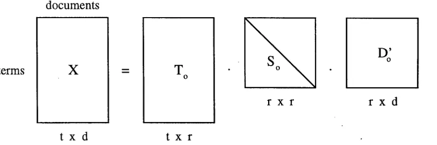
Figure 1: Singular value decomposition (SVD) of matrix X produces matrices T, S and D'.

contain words with different parts of speech. The Bayesian component is used to predict t h e correct word from among same part-of-speech words.

Golding and Schabes selected 18 confusion sets from a list of commonly confused words plus a few that represent typographical errors. T h e y trained their system using a random 80% of the Brow[/corpus (Ku~era and Francis, 1967). The remaining 20% of the corpus was used to test how well the system performed. We have chosen to use the same 18 confusion sets and the Brown corpus in order to compare LSA to Tribayes.

3

L a t e n t S e m a n t i c

Analysis

Latent Semantic Analysis (LSA) was developed at Bellcore for use in information retrieval tasks (for which it is also known as LSI) (Dumais et al., 1988; Deerwester et al., 1990). The premise of the LSA model is t h a t an author begins with some idea or information to be communicated. T h e selection of particular lexical items in a collection of texts is simply evidence for the underlying ideas or information being presented. The goal of LSA, then, is to take the "evidence" (i.e., words) presented and un- cover the underlying semantics of the text passage. Because m a n y words are polysemous (have multiple meanings) and synonymous (have meanings in common with other words), the evidence available in the text tends to be somewhat "noisy." LSA at- tempts to eliminate the noise from the data by first representing the texts in a high-dimensional space and then reducing the dimensionality of the space to only the most i m p o r t a n t dimensions. This process is described in more detail in Dumais (1988) or Deerwester (1990), but a brief description is provided here.

A collection of texts is represented in m a t r i x for- mat. T h e rows of the m a t r i x correspond to terms and the columns represent documents. The individual cell values are based on some function of the term's frequency in the corresponding document and

167

its frequency in the whole collection. T h e function for selecting cell values will be discussed in section 4.2. A singular value decomposition (SVD) is performed on this matrix. SVD factors the original matrix into the product of three matrices. We'll identify these matrices as T, S, and D ' ( s e e Figure 1). The T matrix is a representation of the original term vectors as vectors of derived orthogonal factor values. D ' is a similar representation for the original document vectors. S is a diagonal m a t r i x 2 of rank r. It is also called the singular value matrix. T h e singular values are sorted in decreasing order along the diagonal. T h e y represent a scaling factor for each dimension in the T and D ' matrices.

Multiplying T, S, and D ' t o g e t h e r perfectly repro- duces the original representation of the text collection. Recall, however, t h a t the original representation is expected to be noisy. W h a t we really want is an approximation of the original space t h a t elim- inates the majority of the noise and captures the most important ideas or semantics of the texts.

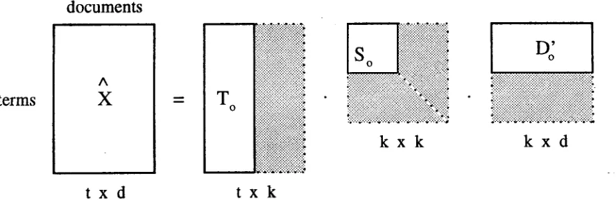
An approximation of the original m a t r i x is created by eliminating some number of the least i m p o r t a n t singular values in S. T h e y correspond to the least important (and hopefully, most noisy) dimensions in the space. This step leaves a new m a t r i x (So) of rank k. 3 A similar reduction is made in T and D by retaining the first k columns of T and the first k rows of D ' as depicted in Figure 2. T h e product

of the resulting

To, So,

and

D'o

matrices is a least

squares best fit reconstruction of the original m a t r i x (Eckart and Young, 1939). T h e reconstructed matrix defines a space that represents or predicts the frequency with which each term in the space would appear in a given document or text segment given

an infinite sample of semantically similar texts

(Lan-

2A diagonal matrix is a square matrix that contains non-zero values only along the diagonal running from the upper left to the lower right.

[image:2.612.87.532.90.238.2]

(3)

t e r m s

documents

A

X

. . .

iiiiiiii ! D: I

::::::::::::::::::::::::::::::::::: !:~:~,~:i:~:i:i,i:~:i:i:!:i:~:~:~

+:.:.:.:.:.:.:.:.:.:.:.:.:.:.:.:*

:::::::::::::::::::::::::::::::::::: . . .

::::::::::::::::::::::::::::::::::::::::::::::::::::::::::::::: :::::::::::::::::::::::::::::::::::::::::::::::::::::::::::::::::::::::::::::::::

:::::::::::::::::::::::::::::::::::

~:~:~:~:~:~:~:~:~:~:~:~:~:~:!:~:~:~ ~: :~: :~:~:i:!:i:i:i:i:i: :i:i:i:~ k x k k x d

t x d

t x k

Figure 2: Results of reducing the T, S and

D'

matrices produced by SVD to rank k. Recombining

the reduced matrices gives X, a least squares best fit reconstruction of the original m a t r i x .

dauer and Dumais, (In press)).

New t e x t passages can be projected into the space by c o m p u t i n g a weighted average of the t e r m vectors which correspond to the words in the new text. In the contextual spelling correction task, we can gen- erate a vector representation for each text passage in which a confusion word appears. T h e similarity between this text passage vector and the confusion word vectors can be used to predict the m o s t likely word given the context or text in which it will appear. '

4 E x p e r i m e n t a l M e t h o d

4.1 D a t a

Separate c o r p o r a for training and testing LSA's abil- ity to correct contextual word usage errors were created f r o m the Brown corpus (Ku~era and Francis, 1967). T h e Brown corpus was parsed into individual sentences which are r a n d o m l y assigned to either a training corpus or a test corpus. Roughly 80% of the original corpus was assigned as the training corpus and the other 20% was reserved as the test corpus. For each confusion set, only those sentences in the training corpus which contained words in the confusion set were extracted for construction of an LSA space. Similarly, the sentences used to test the LSA space's predictions were those extracted f r o m the test corpus which contained words from the confusion set being examined. T h e details of the space construction and testing m e t h o d are described below.

4.2 Training

Training the s y s t e m consists of processing the training sentences and constructing an LSA space from t h e m . LSA requires the corpus to be segmented into documents. For a given confusion set, an LSA space is constructed by treating each training sentence as a document. In other words, each training sentence is used as a column in the LSA m a t r i x . Before be-

ing processed by LSA, each sentence undergoes the following transformations: context reduction, stem- ming, b i g r a m creation, and t e r m weighting.

C o n t e x t r e d u c t i o n is a step in which the sentence is reduced in size to the confusion word plus the seven words on either side of the word or up to the sentence boundary. T h e average sentence length in the corpus is 28 words, so this step has the effect of reducing the size of the d a t a to a p p r o x i m a t e l y half the original. Intuitively, the reduction ought to improve performance by disallowing the distantly located words in long sentences to have any influence on the prediction of the confusion word because t h e y usually have little or nothing to do with the selection of the proper word. In practice, however, the reduction we use had little effect on the predictions obtained from the LSA space.

We ran some experiments in which we built LSA spaces using the whole sentence as well as other context window sizes. Smaller context sizes d i d n ' t seem to contain enough information to produce good predictions. Larger context sizes (up to the size of the entire sentence) produced results which were not sig- nificantly different f r o m the results reported here. However, using a smaller context size reduces the total n u m b e r of unique t e r m s by an average of 13%. Correspondingly, using fewer t e r m s in the initial m a - trix reduces the average running t i m e and s t o r a g e space requirements by 17% and 10% respectively.

S t e m m i n g is the process of reducing each word to its morphological root. T h e goal is to t r e a t the different morphological variants of a word as the same

entity. For example, the words

smile, smiled, smiles,

smiling,

and

smilingly

(all f r o m the corpus) are re-

duced to the root

smile

and t r e a t e d equally. We

tried different s t e m m i n g algorithms and all improved the predictive performance of LSA. T h e results presented in this paper are based on P o r t e r ' s (Porter,

1980) algorithm.

[image:3.612.97.541.92.237.2]

(4)

Bigrams are formed between all adjacent pairs of words. T h e b i g r a m s are treated as additional terms during the LSA space construction process. In other words, the b i g r a m s fill their own row in the LSA m a - trix.

T e r m w e i g h t i n g is an effort to increase the weight or i m p o r t a n c e of certain terms in the high

dimensional space. A local and global weighting

is given to each t e r m in each sentence. T h e local weight is a combination of the raw count of the particular t e r m in the sentence and the t e r m ' s prox- imity to the confusion word. Terms located nearer to the confusion word are given additional weight in a linearly decreasing manner. T h e local weight of each t e r m is then flattened by taking its log2. T h e global weight given to each t e r m is an a t t e m p t to measure its predictive power in the corpus as a whole. We found t h a t entropy (see also (Lochbaum and Streeter, 1989)) performed best as a global measure. Furthermore, t e r m s which did not a p p e a r in more t h a n one sentence in the training corpus were removed.

While LSA can be used to quickly obtain satisfac- tory results, some tuning of the p a r a m e t e r s involved can improve its performance. For example, we chose (somewhat arbitrarily) to retain 100 factors for each LSA space. We wanted to fix this variable for all confusion sets and this n u m b e r gives a good average performance. However, tuning the n u m b e r of factors to select the "best" n u m b e r for each space shows an average of 2% i m p r o v e m e n t over all the results and up to 8% for some confusion sets.

4.3 T e s t i n g

Once the LSA space for a confusion set has been created, it can be used to predict the word (from the confusion set) m o s t likely to appear in a given sentence. We tested the predictive accuracy of the LSA space in the following manner. A sentence from the test corpus is selected and the location of the confusion word in the sentence is treated as an unknown word which m u s t be predicted. One at a time, the w o r d s f r o m the confusion set are inserted into the sentence at the location of the word to be predicted and the s a m e t r a n s f o r m a t i o n s t h a t the training sentences undergo are applied to the test sentence. T h e inserted confusion word is then removed from the sentence (but not the b i g r a m s of which it is a part) because its presence biases the comparison which oc- Curs later. A vector in LSA space is constructed from the resulting terms.

T h e word predicted m o s t likely to appear in a sentence is determined by comparing the similarity of each test sentence vector to each confusion word vector f r o m the LSA space. Vector similarity is evalu- ated by c o m p u t i n g the cosine between two vectors. T h e pair of sentence and confusion word vectors with the largest cosine is identified and the corresponding confusion word is chosen as the m o s t likely word for

169

the test sentence. T h e predicted word is c o m p a r e d to the correct word and a tally of correct predictions is kept.

5 R e s u l t s

T h e results described in this section are based on the 18 confusion sets selected by Golding (1995; 1996). Seven of the 18 confusion sets contain words t h a t are all the same part of speech and the remaining 11 contain words with different parts of speech. Golding and Schabes (1996) have already shown t h a t using a t r i g r a m model to predict words from a confusion set based on the expected p a r t of speech is very effective. Consequently, we will focus m o s t of our atten- tion on the seven confusion sets containing words of the same p a r t of speech. These seven sets are listed first in all of our tables and figures. We also show the results for the remaining 11 confusion sets for comparison purposes, but as expected, these a r e n ' t as good. We, therefore, consider our s y s t e m com- p l e m e n t a r y to one (such as Tribayes) t h a t predicts based on part of speech when possible.

5.1 B a s e l i n e P r e d i c t i o n S y s t e m

We describe our results in t e r m s of a baseline prediction system t h a t ignores the context contained in the test sentence and always predicts the confusion word t h a t occurred most frequently in the training corpus. Table 1 shows the performance of this baseline predictor. T h e left half of the table lists the various confusion sets. T h e next two columns show the training and testing corpus sentence counts for each confusion set. Because the sentences in the Brown corpus are not tagged with a m a r k u p language, we identified individual sentences a u t o m a t i c a l l y based on a small set of heuristics. Consequently, our sentence counts for the various confusion sets differ slightly from the counts reported in (Golding and Schabes, 1996).

T h e right half of Table 1 shows the m o s t frequent word in the training corpus from each confusion set. Following the m o s t frequent word is the baseline performance data. Baseline performance is the percentage of correct predictions m a d e by choosing the given (most frequent) word. T h e percentage of correct predictions also represents the frequency of sentences in the test corpus t h a t contain the given word. T h e final column lists the training corpus frequency of the given word. T h e difference between the baseline performance column and the training corpus frequency column gives some indication a b o u t how evenly distributed the words are between the two corpora.

For example, there are 158 training sentences for

the confusion set

{principal, principle}

and 34 test

sentences. Since the word

principle

is listed in the

(5)

Confusion Set Train Test

principal principle 158 34

raise rise 117 36

affect effect 193 53

peace piece 257 62

country county 389 91

a m o u n t number 480 122

among between 853 203

accept except 189 62

begin being 623 161

lead led 197 63

passed past 353 81

quiet quite 280 76

weather whether 267 67

cite sight site 128 32

it's its 1577 391

than then 2497 578

you're your 734 220

their there they're 4176 978

Most Freq. Base (Train Freq.)

principle 41.2 (57.6)

rise 72.2 (65.0)

effect 88.7 (85.0)

peace 58.1 (59.5)

country 59.3 (71.0)

number 75.4 (73.8)

between 62.1 (66.7)

except 67.7 (73.5)

being 88.8 (89.4)

led 50.8 (52.3)

past 64.2 (63.2)

quite 88.2 (76.1)

whether 73.1 (79.0)

sight 62.5 (54.7)

its 84.7 (84.9)

than 58.8 (55.3)

your 86.8 (84.5)

there 53.4 (53.1)

Table 1: Baseline performance for 18 confusion sets. T h e table is divided into confusion sets containing words of the same part of speech and those which have different parts of speech.

we can see t h a t it occurred in almost 58% of the training sentences. However, it occurs in only 41% of the test sentences and thus the baseline predictor scores only 41% for this confusion set.

5.2 L a t e n t S e m a n t i c A n a l y s i s

Table 2 shows the performance of LSA on the contextual spelling correction task. T h e table provides the baseline performance information for compari-

son to LSA. In all but the case of

{amount, number},

LSA improves upon the baseline performance. The improvement provided by LSA averaged over all confusion sets is about 14% and for the sets with the same part of speech, the average improvement is

16%.

Table 2 also gives the results obtained by Tribayes as reported in (Golding and Schabes, 1996). The baseline performance given in connection with Trib- ayes corresponds to the partitioning of the Brown corpus used to test Tribayes. It. should be noted that. we did not implement Tribayes nor did we use the same partitioning of the Brown corpus as Tribayes. Thus, the comparison between LSA and Tribayes is an indirect one.

T h e differences in the baseline predictor for each system are a result of different partitions of the

Brown corpus. Both systems randomly split the

data such t h a t roughly 80% is allocated to the training corpus and the remaining 20% is reserved for the test corpus. Due to the random nature of this process, however, the corpora must differ between the two systems. T h e baseline predictor presented in this paper and in (Golding and Schabes, 1996) are based on the same method so the correspond-

ing columns in Table 2 can be compared to get an idea of the distribution of sentences t h a t contain the most frequent word for each confusion set.

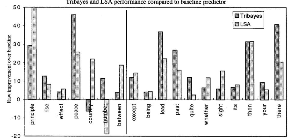
Examination of Table 2 reveals t h a t it is difficult to make a direct comparison between the results of LSA and Tribayes due to the differences in the partitioning of the Brown corpus. Each system should perform well on the most frequent confusion word in the training data. Thus, the distribution of the most frequent word between the the training and the test corpus will affect the performance of the system. Because the baseline score captures information about the percentage of the test corpus t h a t should be easily predicted (i.e., the portion t h a t contains the most frequent word), we propose a comparison of the results by examination of the respec- tive systems' improvement over the baseline score reported for each. The results of this comparison are charted in Figure 3. T h e horizontal axis in the figure represents the baseline predictor performance for each system (even though it varies between the two systems). The vertical bar thus represents the performance above (or below) the baseline predictor for each system on each confusion set.

LSA performs slightly better, on average, than Tribayes for those confusion sets which contain words of the same part of speech. Tribayes clearly out-performs LSA for those words of a different part

of speech. Thus, LSA is doing better than the

[image:5.612.170.491.88.303.2]

(6)

LSA Tribayes

Confusion Set Baseline LSA Baseline Tribayes

principal principle raise rise

affect effect peace piece country county amount number among between accept except begin being lead led passed past quiet quite weather whether cite sight site it's its than then you're your their there they're

41.2 91.2

72.2 80.6

88.7 94.3

58.1 83.9

59.3 81.3

75.4 56.6

62.1 80.8

67.7 82.3

88.8 93.2

50.8 73.0

64.2 80.3

88.2 90.8

73.1 85.1

62.5 78.1

84.7 92.8

58.8 90.5

86.8 91.4

53.4 73.9

58.8 88.2

64.1 76.9

91.8 95.9

44.0 90.0

91.9 85.5

71.5 82.9

71.5 75.3

70.0 82.0

93.2 97.3

46.9 83.7

68.9 95.9

83.3 95.5

86.9 93.4

64.7 70.6

91.3 98.1

63.4 94.9

89.3 98.9

56.8 97.6

Table 2: LSA performance for 18 confusion sets. The results of Tribayes (Golding and Schabes,

1996) are also given.

5 0

4 0

o

o 2 0

~ 1 0

-10

- 2 0

Tribayes and L S A performance compared to baseline predictor

[ ] Tribayes [ ] LSA

:2

!!i! ~ ...=

!!!i !:!::!

:5: :.:.:.-

fill i:~:~:

>:.

0 " 0 - - 0 ~ ¢.~ " - - ~ t - . - - O'J " - - t'-" 0 (I)

0 • Z~ X ~ ~ ~ ~ '~ ~ ¢-

.__=_ " ~ o_ o *~ • = * "

o _ o

Figure 3: Comparison of Tribayes vs. LSA performance above the baseline metric.

[image:6.612.188.461.118.341.2] [image:6.612.78.558.450.680.2]

(7)

a Bayesian classifier for making predictions a m o n g words of the s a m e p a r t of speech.

5.3 P e r f o r m a n c e T u n i n g

T h e results t h a t have been presented here are based on uniform t r e a t m e n t for each confusion set. T h a t is, the initial d a t a processing steps and LSA space construction p a r a m e t e r s have all been the same. How- ever, the model does not require equivalent treat- m e n t of all confusion sets. In theory, we should be able to increase the performance for each confusion set by tuning the various p a r a m e t e r s for each confusion set.

In order to explore this idea further, we selected

the confusion set {amount, number} as a testbed

for p e r f o r m a n c e tuning to a particular confusion set. As previously mentioned, we can tune the n u m b e r of factors to a particular confusion set. In the case of this confusion set, using 120 factors increases the p e r f o r m a n c e by 6%. However, tuning this p a r a m - eter alone still leaves the performance short of the baseline predictor.

A quick e x a m i n a t i o n of the context in which b o t h words a p p e a r reveals t h a t a significant percentage (82%) of all training instances contain either the bi-

g r a m of the confusion word preceded by the, fol-

lowed by of, or in some cases, both. For exam-

ple, there are m a n y instances of the collocation

the+humber+of in the training data. However, there are only one third as m a n y training instances for

amount (the less frequent word) as there are for

number. T h i s situation leads LSA to believe t h a t the

b i g r a m s the+amount and amount+of have more dis-

crimination power t h a n the corresponding b i g r a m s

which contain number. As a result, LSA gives t h e m

a higher weight and LSA almost always predicts

amount when the confusion word in the test sentence a p p e a r s in this context. This local context is a poor predictor of the confusion word and its presence tends to d o m i n a t e the decision m a d e by LSA.

By eliminating the words the and of from the train-

ing and testing process, we p e r m i t the remaining context to be used for prediction. T h e elimination of the poor local context combined with the larger n u m b e r of factors increases the performance of LSA to 13% above the baseline predictor (compared to 11% for Tribayes). This is a net increase in performance of 32%!

6 C o n c l u s i o n

We've shown t h a t LSA can be used to attack the p r o b l e m of identifying contextual misuses of words, particularly when those words are the same part of speech. It has proven to be an effective alternative to Bayesian classifiers. Confusions sets whose words are different parts of speech are more effectively han- dled using a m e t h o d which incorporates the word's p a r t of speech as a feature. We are exploring tech-

niques for introducing p a r t of speech information into the LSA space so t h a t the s y s t e m can m a k e better predictions for those sets on which it doesn't yet measure up to Tribayes. We've also shown t h a t for the cost of e x p e r i m e n t a t i o n with different p a r a m - eter combinations, LSA's performance can be tuned for individual confusion sets.

While the results of this experiment look very nice, they still d o n ' t tell us anything a b o u t how useful the technique is when applied to unedited text. T h e testing procedure assumes t h a t a confusion word m u s t be predicted as if the author of the t e x t h a d n ' t supplied a word or t h a t writers misuse the confusion words nearly 50% of the time. For example, consider

the case of the confusion set {principal, principle}.

T h e LSA prediction accuracy for this set is 91%. However, it might be the case t h a t , in practice, peo- ple tend to use the Correct word 95% of the time. LSA has thus introduced a 4% error into the writing process. Our continuing work is to explore the error rate t h a t occurs in unedited text as a m e a n s of as- sessing the "true" performance of contextual spelling correction systems.

7 A c k n o w l e d g m e n t s

T h e first author is supported under D A R P A con- tract SOL BAA95-10. We gratefully acknowledge the c o m m e n t s and suggestions of T h o m a s Landauer and the a n o n y m o u s reviewers.

R e f e r e n c e s

Scott Deerwester, Susan T. Dumais, George W. Fur- haS, T h o m a s K. Landauer, and Richard A. Harsh- man. 1990. Indexing by Latent Semantic Analy-

sis. Journal of the American Society for Informa-

tion Science, 41(6):391-407, September.

Susan T. Dumais, George W. Furnas, T h o m a s K. Landauer, Scott Deerwester, and Richard Harsh- man. 1988. Using Latent Semantic Analysis to

improve access to textual information. In Human

Factors in Computing Systems, CHI'88 Confer- ence Proceedings (Washington, D.C.), pages 281- 285, New York, May. ACM.

Carl Eckart and Gale Young. 1939. A principle

axis t r a n s f o r m a t i o n for n o n - h e r m i t i a n matrices.

American Mathematical Society Bulletin, 45:118- 121.

Peter W. Foltz. 1995. I m p r o v i n g h u m a n -

proceedings interaction: Indexing the C H I index. In Human Factors in Computing Systems: CHI'95 Conference Companion, pages 101-102. Associa- tions for C o m p u t i n g Machinery (ACM), May. William A. Gale, Kenneth W. Church, and David

Yarowsky. 1992. A m e t h o d for d i s a m b i g u a t i n g

word senses in a large corpus. Computers and the

(8)

Andrew R. Golding. 1995. A Bayesian hybrid method for context-sensitive spelling correction. In Proceedings of the Third Workshop on Very Large Corpora, Cambridge, MA.

Andrew R. Golding and Yves Schabes. 1996. Com- bining trigram-based and feature-based methods

for context-sensitive spelling correction. In Pro-

ceedings of the 34th Annual Meeting of the Associ- ation for Computational Linguistics, Santa Clara, CA, June. Association for Computational Linguis- tics.

Karen Kukich. 1992a. Spelling correction for the

telecommunications network for the deaf. Com-

munications of the ACM, 35(5):80-90, May.

Karen Kukich. 1992b. Techniques for automatically

correcting words in text. A CM Computing Sur-

veys, 24(4):377-439, Dec.

Henry KuSera and W. Nelson Francis. 1967. Com-

putational Analysis of Present-Day American En- glish. Brown University Press, Providence, RI. Thomas K. Landauer and Susan T. Dumais. (In

press). A solution to Plato's problem: The La- tent Semantic Analysis theory of acquisition, in-

duction, and representation of knowledge. Psy-

chological Review.

Karen E. Lochbaum and Lynn A. Streeter. 1989. Comparing and combining the effectiveness of La- tent Semantic Indexing and the ordinary vector

space model for information retrieval. Informa-

tion Processing CJ Management, 25(6):665-676. Susan W. McRoy. 1992. Using multiple knowledge

sources for word sense disambiguation. Computa-

tional Linguistics, 18(1):1-30, March.

M. F. Porter. 1980. An algorithm for suffix strip-

ping. Program, 14(3):130-137, July.

Lynn A. Streeter and Karen E. Lochbaum. 1988. An expert/expert-locating system based on au- tomatic representation of semantic structure. In

Proceedings of the Fourth Conference on Artifi- cial Intelligence Applications, pages 345-350, San Diego, CA, March. IEEE.

David Yarowsky. 1994. Decision lists for lexical am- biguity resolution: Application to accent restora-

tion in Spanish and French. In Proceedings of the

32nd Annual Meeting of the Association for Com- putational Linguistics, pages 88-95, Las Cruces, NM, June. Association for Computational Lin- guistics.