Efficient Transformation Based Parsing

(1)

Efficient Transformation-Based Parsing

Giorgio

S a t t a E r i c B r i l l

D i p a r t i m e n t o di E l e t t r o n i c a e d I n f o r m a t i c a D e p a r t m e n t o f C o m p u t e r S c i e n c e U n i v e r s i t £ di P a d o v a J o h n s H o p k i n s U n i v e r s i t y

v i a G r a d e n i g o , 6 / A B a l t i m o r e , M D 2 1 2 1 8 - 2 6 9 4 2-35131 P a d o v a , I t a l y b r i l l © c s , j h u .

edu

satta@dei, unipd, it

A b s t r a c t

In transformation-based parsing, a finite sequence of tree rewriting rules are checked for application to an input structure. Since in practice only a small percentage of rules are applied to any particular structure, the naive parsing algorithm is rather ineffi- cient. We exploit this sparseness in rule applications to derive an algorithm two to three orders of magnitude faster than the standard parsing algorithm.

1 I n t r o d u c t i o n

The idea of using transformational rules in natural language analysis dates back at least to Chore- sky, who a t t e m p t e d to define a set of transformations that would apply to a word sequence to map it from deep structure to surface structure (see (Chomsky, 1965)). Transformations have also been used in much of generative phonology to cap- ture contextual variants in pronunciation, starting with (Chomsky and Halle, 1968). More re- cently, transformations have been applied to a di- verse set of problems, including part of speech tagging, pronunciation network creation, prepositional phrase a t t a c h m e n t disambiguation, and parsing, under the paradigm of transformation-based error-driven learning (see (Brill, 1993; Brill, 1995) and (Brill and Resnik, 1994)). In this paradigm, rules can be learned automatically from a training corpus, instead of being written by hand.

Transformation-based systems are typically deterministic. Each rule in an ordered list of rules is applied once wherever it can apply, then is discarded, and the next rule is processed until the last rule in the list has been processed. Since for each rule the application algorithm must check for a matching at all possible sites to see whether the rule can apply, these systems run in

O(rrpn)

time, where 7r is the number of rules, p is the cost of a single rule matching, and n is the size of the input structure. While this results in fast processing, it is possible to create much faster systems. In (Roche and Schabes, 1995),

a method is described for converting a list of transformations that operates on strings into a deterministic finite state transducer, resulting in an optimal tagger in the sense that tagging requires only one state transition per word, giving a linear time tagger whose run-time is independent of the number and size of rules.

In this paper we consider transformation-based parsing, introduced in (Brill, 1993), and we im- prove upon the

O(Trpn)

time upper bound.. In transformation-based parsing, an ordered sequence of tree-rewriting rules (tree transformations) are applied to an initial parse structure for an input sentence, to derive the final parse structure. We observe that in most transformation-based parsers, only a small percentage of rules are actually applied, for any particular input sentence. For example, in an application of the transformation-based parser described in (Brill, 1993), 7r = 300 rules were learned, to be applied at each node of the initial parse structure, but the average number of rules that are successfully applied at each node is only about one. So a lot of time is spent testing whether the conditions are met for applying a transformation and finding out that they are not met. This paper presents an original algorithm for transformation-based parsing working in

O(ptlog(t))

time, where t is the total number of rules applied for an input sentence. Since in practical cases t is smaller than n and we can neglect the log(n) factor, we have achieved a

time

improvement of a factor of r . We emphasize that rr can be several hundreds large in actual systems where transformations are lexicalized.

Our result is achieved by preprocessing the transformation list, deriving a finite state, determiflistic tree automaton. The algorithm then exploits the au- t o m a t o n in a way that obviates the need for checking the conditions of a rule when that rule will not apply, thereby greatly improving parsing run-time over the straightforward parsing algorithm. In a sense, our algorithm spends time only with rules that can be applied, as if it knew in advance which rules cannot be applied during the parsing process.

(2)

lows. In Section 2 we introduce some preliminaries, and in Section 3 we provide a representation of transformations that uses finite state, deterministic tree a u t o m a t a . Our algorithm is then specified in Sec- tion 4. Finally, in Section 5 we discuss related work in the existing literature.

2

P r e l i m i n a r i e s

We review in the following subsections some terminology t h a t is used t h r o u g h o u t this paper.

2.1 T r e e s

We consider ordered trees whose nodes are assigned labels over some finite alphabet E; this set is denoted as ET. Let T E S T. A node of T is called l e f t m o s t if it does not have any left sibling ( a root node is a leftmost node). The h e i g h t of T is the length of a longest p a t h from the root to one of its leaves (a tree composed of a single node has height zero). We define I T I as the number of nodes in T. A tree T E y]T is denoted as A if it consists of a single leaf node labeled by A, and as A(T1,T2,... ,Ta), d >_ 1,

if T has root labeled by A with d (ordered) children denoted by T 1 , . . . , T d . Sometimes in the examples we draw trees in the usual way, indicating each node with its label.

W h a t follows is standard terminology from the tree pattern m a t c h i n g literature, with the simplifi- cation t h a t we do not use variable terms. See (Hoff- m a n n and O'Donnell, 1982) for general definitions. Let n be a node of T. We say that a tree S m a t c h e s T at n if there exists a one-to-one mapping from the nodes of S to the nodes of T, such that the following conditions are all satisfied: (i) if n' maps to n",

then n ~ and n I~ have the same label; (ii) the root of S maps to n; and (iii) if n ~ maps to n" and n ~ is not a leaf in S, then n ~ and n" have the same degree and the i-th child of n ~ maps to the i-th child of n% We say that T and S are e q u i v a l e n t if they match each other at the respective root nodes. In what follows trees t h a t are equivalent are not treated as the same object. We say t h a t a tree T ' is a s u b t r e e of T at n if there exists a tree S that matches T at n, and T ~ consists of the nodes of T t h a t are matched by some node of S and the arcs of T between two such nodes. We also say that T ' is matched by S at n. In addition, T ' is a p r e f i x of T if n is the root of T; T ' is the suffix of T at n if T ' contains all nodes of T dominated by n.

E x a m p l e 1 Let T -- B(D, C(B(D, B), C)) and let n be the second child of T's root. S -- C ( B , C )

matches T at n. S' = B(D, C(B), C)) is a prefix o r S and S" = C(B(D, B), C) is the suffix of T at n. [] We now introduce a tree replacement operator t h a t will be used throughout the paper. Let S be a subtree of T and let S / be a tree having the same number of leaves as S. Let nl, n2, • . . , nz and

n~,n~,...,n~, 1 > 1, be all the leaves from left to

B

D C_

B_ E I

E

B

E

B

C B

f

D E

Figure 1: From left to right, top to b o t t o m : tree T with subtree S indicated using underlined labels at its nodes; tree S' having the same number of leaves as S; tree T [ S / S ~] obtained by "replacing" S with S ~.

right of S and S', respectively. We write T[S/S']

to denote the tree obtained by embedding S ~ within T in place of S, through the following steps: (i) if the root of S is the i-th child of a node n] in T, the root of S I becomes the i-th child of n] ; and (ii) the (ordered) children of n~ in T, if any, become the children of n~, 1 < i < l. T h e root of T [ S / S ~] is the root of T if node n] above exists, and is the root of S t otherwise.

E x a m p l e 2 Figure 1 depicts trees T, S I and T ~ in this order. A subtree S of T is also indicated using underlined labels at nodes of T. Note t h a t S and S' have the same number of leaves. Then we have

T' = T[S/S']. n

2 . 2 T r e e a u t o m a t a

Deterministic (bottom-up) tree a u t o m a t a were first introduced in (Thatcher, 1967) (called F R T there). The definition we propose here is a generalization of the canonical one to trees of any degree. Note t h a t the transition function below is c o m p u t e d on a number of states that is independent of the degree of the input tree. Deterministic tree a u t o m a t a will be used later to implement the b o t t o m - u p tree pattern matching algorithm of (Hoffmann and O'- Donnell, 1982).

D e f i n i t i o n 1 A deterministic tree automaton (DTA)

is a 5-tuple M = (Q, ~, ~, qo, F), where Q is a finite set of s~ates, ~ is a finite alphabet, qo E Q is the initial state, F C Q is the set of final states and 6 is a transition function mapping Q~ × E into O.

[image:2.612.325.543.69.240.2]

(3)

reached upon reading the immediate left sibling and the rightmost child of the current node, if any. In this way the decision of the DTA is affected not only by the portion of the tree below the currently read node, but also by each subtree rooted in a left sibling of the current node. This is formally stated in what follows. Let T E ~T and let n be one of its nodes, labeled by a. T h e state r e a c h e d by M upon reading n is recursively specified as:

6 ( T , n ) = ~ ( X , X ' , a ) , (1)

where X -- q0 if n is a leftmost node, X -- 6(T, n') if n' is the immediate left sibling of n; and X ' -- q0 if n is a leaf node, X ' = 6(T, n") if n " is the rightmost child of n. T h e tree language recognized by M is the set

L ( M ) = { T [ ~(T, n) E F, T E E T, n the root of T}. (2)

E x a m p l e 3 Consider the infinite set L = { B ( A , C), B ( A , B ( A , C)), B ( A , B ( A , B ( A , C ) ) ) , . . . } consisting of all right-branching trees with internal nodes labeled by B and with strings A'~C, n > 1 as their yields. Let M = (Q, { A , B , C } , 6, qo, {qBc}) be a DTA specified as follows: Q = {q0, qA, qnc, q - i } ; 6(qo, qo,A) = qA, 6(qA,qo, C) = 5(qA, qBC, B) = qBC and q - i is the value of all other entries of 5. It is not difficult to see that L ( M ) = L. 1:3

Observe that when we restrict to monadic trees, that is trees whose nodes have degree not greater than one, the above definitions correspond to the well known formalisms of deterministic finite state au- t o m a t a , the associated extended transition function, and the regular languages.

2.3 T r a n s f o r m a t i o n - b a s e d p a r s i n g

Transformation-based parsing was first introduced in (Brill, 1993). Informally, a transformation-based parser assigns to an input sentence an initial parse structure, in some uniform way. Then the parser iteratively checks an ordered sequence of tree transformations for application to the initial parse tree, in order to derive the final parse structure. This results in a deterministic, linear time parser. In order to present our algorithm, we abstract away from the assignment of the initial parse to the input, and introduce below the notion of transformation- based tree rewriting system. The formulation we give here is inspired by (Kaptan and Kay, 1994) and (Roche and Schabes, 1995). The relationship between transformation-based tree rewriting systems and standard term-rewriting systems will be discussed in the final section.

D e f i n i t i o n 2 A transformation-based tree rewriting system ( T T S ) is a pair G = ( E , R ) , where ~ is a finite alphabet and R = ( r i , r 2 , . . . , r ~ ) , 7r >_ 1, is a finite sequence of tree rewriting rules having the

form Q --+ Q', with Q, Q' E ~T and such that Q and Q' have the same number of leaves.

If r = (Q ~ Q'), we write lhs(r) for Q and rhs(r) for Q'. We also write lhs(R) for {lhs(r) I r E R}. (Recall that we regard lhs(r/) and lhs(rj), i # j , as different objects, even if these trees are equivalent.) We define [r I = Ilhs(r) l + I rhs(r) I.

The notion of transformation associated with a T T S G = (E, R) is now introduced. Let C, C ' E E T. For any node n of C and any rule r = (Q ~ Q') of G, we write

C ~

C'

(3)

if Q does not match C at n and C = C'; or if Q matches C at n and C ' = C[S/Q'], where S is the subtree of T matched by Q at n and Q'c is a fresh copy of Q'. Let < n l , n 2 , . . . , n t l , t > 1, be the post- ordered sequence of all nodes of C. We write

C ~ C ' (4)

r , n •

if C i - i ~ Ci, 1 < i <_ t, Co = C and Ct = C'. Finally, we define the translation induced by G on Ea, as the map M ( G ) = { ( C , C ' ) I C E

y]T, Ci_I~:~C i

for 1 < i < ~r, Co = C , C~ = C ' } .

3 R u l e r e p r e s e n t a t i o n

We develop here a representation of rule sequences that makes use of DTA and that is at the basis of the main result of this paper. Our technique im- proves the preprocessing phase of a b o t t o m - u p tree pattern matching algorithm presented in (Hoffmann and O'Donnell, 1982), as it will be discussed in the final section.

Let G = ( ~ , R ) be a T T S , R = ( r i , r 2 , . . . , r ~ ) . In what follows we construct a DTA that "detects" each subtree of an input tree that is equivalent to some tree in lhs(_R). We need to introduce some additional notation. Let N be the set of all nodes from the trees in lhs(R). Call Nr the set of all root nodes (in N), N,~ the set of all leftmost nodes, Nz the set of all leaf nodes, and Na the set of all nodes labeled by a E ~. For each q E 2 N, let right(q) = {n I n E N, n' E

q, n has immediate left sibling n'} and let up(q) = {n [ n E N, n' E q, n h a s r i g h t m o s t c h i l d n ' } . Also, let q0 be a fresh symbol.

D e f i n i t i o n 3 G is associated with a DTA A a = (2 N U {q0}, E, 6a, qo, F), where F = {q [ q E

2 N, (q f3 Nr) # 0} and 6G is specified as follows:

(i) 5a(qo,qo,a) = No M Nm A N t ;

(it) dia(qo,q',a) = N a A N m A ( N t U u p ( q ' ) ) , f o r q ' # qo;

(iii) diG(q, qo, a) = Na A Nz t] (Nr U right(q)), for q qo;

(4)

Observe t h a t each state of A c simultaneously car- ries over the recognition of several suffixes of trees in lhs(/~). These processes are started whenever A c reads a leftmost node n with the same label as a leftmost leaf node in some tree in lhs(R) (items (i) and (ii) in Definition 3). Note also t h a t we do not require any m a t c h i n g of the left siblings when we m a t c h the root of a tree in lhs(R) (items (iii) and (iv)).

B B

A --~

a

B

A / ' D

B

A

c B

- + c c A

A B

B B

C B A B

A B

Figure 2: F r o m top to b o t t o m : rules r l , r2 and r3 of G.

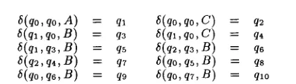
E x a m p l e 4 Let G = ( E , R ) , where E = {A, B, C, D} and R = (rl,r2, r3). Rules ri are depicted in Figure 2. We write nij to denote the j - t h node • in a post-order e n u m e r a t i o n of the nodes of lhs(ri), 1 < i < 3 and 1 < j <__ 5. (Therefore n35 denotes the root node of lhs(r3) and n22 denotes the first child of the second child of the root node of lhs(r~).) If we consider only the useful states, t h a t is those states t h a t can be reached on an actual input, the D T A A c --- (Q, E, 5, qo, F ) , is specified as follows: Q = {qi I 0 < i < I1}, where ql = {nll,n12, n22, n32}, q2 = {n21,n3x}, q3 = {n13, n23}, q4 = {n33}, q5 = {n14}, q6 = {n24}, q7 = {n34}, qs = {n15}, q9 -= {n35}, qlo = {n25}, qll = (b; F = {qs, qg, qlo}. T h e transition function 5, restricted to the useful states, is specified in Figure 3. Note t h a t a m o n g the 215 + 1 possible states, only 12 are useful. []

6 ( q o , q o , A ) = ql 6 ( q o , q o , C ) = q2 6(qa,qo, B ) = q3 6 ( q l , q o , C ) = q, 6 ( q l , q z , B ) = qs 6(q2, q 3 , B ) = qs ~(q~,q,, B ) = q7 ~(qo, qs, B ) = q~

6 ( q o , q 6 , B ) = q9 6(qo, q T , B ) = qlo

Figure 3: Transition function of G. For all (q, q~, a) E Q2× E not indicated above, 5(q, q', a) = qll-

Although the n u m b e r of states of A c is exponen-

tial in I N I, in practical cases m o s t of these states are never reached by the a u t o m a t o n on an actual input, and can therefore be ignored. This h a p p e n s whenever there are few pairs of suffix trees of trees in lhs(R) t h a t share a c o m m o n prefix tree b u t no tree in the pair matches the other at the root node. This is discussed at length in (Hoffmann and O ' D o n - nell, 1982), where an u p p e r bound on the n u m b e r of useful states is provided.

T h e following l e m m a provides a characterization of A a t h a t will be used later.

L e m m a 1 Let n be a node o f T E ~T and let n ~ be the roof node of r E R. Tree lhs(r) matches T a f n if and only if n' E i G ( T , n ) .

P r o o f ( o u t l i n e ) . T h e s t a t e m e n t can be shown by proving the following claim. Let m be a node in T and m t be a node in lhs(r). Call m l , . . . , m ~ = m, k > 1, the ordered sequence of the left siblings of m, with m included, and call m ~ , . . . , m' k, -" m', k' > 1, the ordered sequence of the left siblings of m ~, with m ' included. If m ' ~ N r , then the two following conditions are equivalent:

* m ' E i v ( T , m);

• k = k' and, for 1 < i < k, the suffix of lhs(r) at m~ m a t c h e s T at mi.

T h e claim can be shown by induction on the posi- tion of m ~ in a post-order e n u m e r a t i o n of the nodes of lhs(r). T h e l e m m a then follows f r o m the specification of set F and the t r e a t m e n t of set N~ in items (iii) and (iv) in Definition 3. []

We also need a function m a p p i n g F x { 1 . . ( r + 1)} into {1..r} U {.1_}, specified as (min@ =_1_):

next(q,i) = m i n { j [ i < j < 7r, lhs(rj) has root node in q}. (5)

Assume t h a t q E F is reached by AG u p o n reading a node n (in some tree). In the next section next(q, i) is used to select the index of the rule t h a t should be next applied at node n, after the first i - 1 rules of R have been considered.

4 T h e a l g o r i t h m

We present a translation a l g o r i t h m for T T S t h a t can i m m e d i a t e l y be converted into a t r a n s f o r m a t i o n - based parsing algorithm. We use all definitions introduced in the previous sections. To simplify the presentation, we first m a k e the a s s u m p t i o n t h a t the order in which we apply several instances of the s a m e rule to a given tree does not affect the outcome. Later we will deal with the general case.

4.1 O r d e r - f r e e c a s e

[image:4.612.84.308.183.336.2] [image:4.612.91.304.590.651.2]

(5)

of a tree in lhs(R). Given trees T and S, S a subtree of T, we write local(T, S) to denote the set of all nodes of S and the first h a proper ancestors of the root of S' in T (when these nodes are defined).

L e m m a 2 Assume that lhs(r), r E R, matches a tree T at some node n. Let T ~'~ T' and lel S be the copy of rhs(r) used in the rewriting. For every node n' no~ included in local(T', S), we have ~a(T, n') = Oa(T',n'). []

We precede the specification of the m e t h o d with an informal presentation. T h e following three d a t a structures are used. An associative list state associates each node n of the rewritten input tree with the state reached by A a upon reading n. If n is no longer a node of the rewritten input tree, state

associates n with the emptyset. A set rule(i) is associated with each rule ri, containing some of the nodes of the rewritten input tree at which lhs(ri) matches. A heap d a t a structure H is also used to order the indices of the n o n - e m p t y sets rule(i) according to the priority of the associated rules in the rule sequence. All the above d a t a structures are updated by a procedure called update.

To c o m p u t e the translation M ( G ) we first visit the input tree with AG and initialize our d a t a structures in the following way. For each node n, state is assigned a state of AG as specified above. If rule ri m u s t be applied first at n, n is added to rule(i) and H is updated. We then enter a m a i n loop and re- trieve elements f r o m the heap. When i is retrieved, rule ri is considered for application at each node n in rule(i). It is i m p o r t a n t to observe that, since some rewriting of the input tree might have occurred in between the t i m e n has been inserted in rule(i) and the time i is retrieved from H , it could be t h a t the current rule ri can no longer be applied at n. I n f o r m a t i o n in state is used to detect these cases. Crucial to the efficiency of our algorithm, each time a rule is applied only a small portion of the current tree needs to be reread by AG, in order to u p d a t e our d a t a structures, as specified by L e m m a 2 above. Finally, the m a i n loop is exited when the heap is empty.

A l g o r i t h m l Let G - ( ~ , R ) be a T T S , R = ( r l , r 2 , . . . , r ~ ) . a n d l e t T E ~ be an input tree. Let A a = (2 ~ U {q0}, ~, ~a, q0, F ) be the DTA associated with G and ~G the reached state function. Let also i be an integer valued variable, state be an associative array, rule(i) be an initially e m p t y set, for 1 < i < ~', and let H be a heap d a t a structure. (n ---+ rule(i) adds n to rule(i); i ---* H inserts i in H ; i ~-- H assigns to i the least element in H , i f H is not empty.) T h e algorithm is specified in Figure 4. []

E x a m p l e 4 (continued) We describe a run of Al- g o r i t h m 1 working with the sample T T S G = (E, R) previously specified (see Figure 2).

p r o c update( oldset, newset, j) for each node n E oldset

state(n) ~ O

for each node n E newset do state(n) ~- gG(C, n)

if state(n) • F and next(state(n), j) #.l_ then do if rule(next(state(n), j) ) = O

then next(state(n), j) --~ Y

n ~ rule(next(state(n), j ) ) od

od

main

C + - - T ; i , - 1

update(O, nodes of C, i)

while H not empty do i ~ - H

for each node n E rule(i) s.t. the root of lhs(ri) is in state(n) do

S ~ the subtree of C matched by lhs(ri) at n S I *-- copy of rhs(ri)

c ,-- c [ s / s ' ]

update(node~ of S, lo~al(C, S'), i + 1)

od od return C.

Figure 4: Translation algorithm c o m p u t i n g M ( G ) for a T T S G.

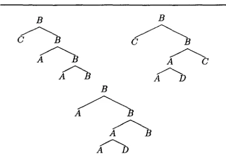
Let Ci E ~T, 1 < i < 3, be as depicted in Figure 5. We write mij to denote the j - t h node in a post- order enumeration of the nodes of Ci, 1 < i < 3 and 1 < j < 7. Assume t h a t CI is the input tree.

After the first call to procedure update, we have state(m17) = qz0 = {n25} and state(m16) = qs = {nzh}; no other final state is associated with a node of C1. We also have t h a t r u l e ( l ) = {m16}, rule(2) = {m17}, rule(3) = 0 and H contains indices 1 and 2. Index 1 is then retrieved f r o m H and the only node in rule(l), i.e., mr6, is considered. Since the root of lhs(rz), i.e., node n15, belongs to q8, mz~ passes the test in the head of the for-statement in the main program. T h e n rz is applied to C1, yielding C2. Observe t h a t m l l = m21 and m17 - - m27; all the remaining nodes of C2 are fresh nodes.

T h e next call to update, associated with the application of r l , updates the associative list state in such a way t h a t state(m27) = q9 = { n 3 5 } , and no other final state is associated with a node of C2. Also, we now have rule(l) = {m16}, r u l e ( 2 ) = {m27} (recall t h a t m 1 7 = m 2 7 ) , rule(3) = {m27}, and H contains indices 2 and 3.

[image:5.612.298.519.66.336.2]

(6)

B

C B

A B

B

C B

A C

A D

B

A B

A

A D

Figure 5: F r o m left to right, top to b o t t o m : trees C1, C2 and C3. In the sample T T S G we have (C1, C3) E

M(G),

since C1 ~=~ C~ ~=~ C2 ~=~ Ca.

m a i n p r o g r a m is not executed this time.

Finally, index 3 is retrieved f r o m H and node m27 is again considered, this t i m e for the application of rule r3. Since the root of lhs(ra), i.e., node n35, belongs to

state(m27), r3

is applied to C2 at node m27, yielding C3. D a t a structures are again u p d a t e d by a call to procedure

update

with the second p a r a m - eter equal to 4. T h e n state qs is associated with node

m37,

the root node of C3. Despite of the fact t h a t qs E F , we now have

next(qs,

4) = _k. There- fore rule rl is not considered for application to C3. Since H is now empty, the c o m p u t a t i o n terminates returning C3. []

T h e results in L e m m a 1 and L e m m a 2 can be used to show that, in the m a i n p r o g r a m , a node n passes the test in the head of the for-statement if and only if lhs(ri) m a t c h e s C at n. T h e correctness of Algo- r i t h m 1 then follows f r o m the definition of the heap d a t a structure.

We now turn to c o m p u t a t i o n a l complexity issues. Let p = maxl<i<_~lril. For T e E T, let a l s o t ( T ) be the total n u m b e r of rules t h a t are successfully applied on a run of Algorithm i on input T, counting repetitions.

T h e o r e m 1

The running time of Algorithm 1 on

input tree T is

0 ( I

TI + pt(T)

log(t(T))).

P r o o f . We can i m p l e m e n t our d a t a structures in such a way t h a t each of the primitive access operations t h a t are executed by the algorithm takes a constant a m o u n t of time.

Consider each instance of the m e m b e r s h i p of a node n in a set

rule(i)

and represent it as a pair (n, i). We call

active

each pair (n, i) such t h a t lhs(ri) matches C at n at the t i m e i is retrieved f r o m H . As already mentioned, these pairs pass the test in the head of the for-loop in the m a i n program. T h e number of active pairs is therefore

t(T).

All remaining

pairs are called

dead.

Note t h a t an active pair (n, i) can turn at m o s t I l h s ( r i ) I + h R active pairs into dead ones, through a call to the procedure

update.

Hence the total n u m b e r of dead pairs m u s t be

O(pt(T)).

We conclude t h a t the n u m b e r of pairs t o t a l l y instantiated by the algorithm is

O(pt(T)).

It is easy to see t h a t the n u m b e r of pairs totMly instantiated by the algorithm is also a b o u n d on the n u m b e r of indices inserted in or retrieved f r o m the heap. T h e n the t i m e spent by the a l g o r i t h m with the heap is

O(pt(T)

log(t(T))) (see for instance (Cor- men, Leiserson, and Rivest, 1990)). T h e first cMl to the procedure

update

in the m a i n p r o g r a m takes t i m e proportional to ]T[. All r e m a i n i n g operations of the algorithm will now be charged to some active pair.

For each active pair, the b o d y of the for-loop in the mMn p r o g r a m and the b o d y of the

update

procedure are executed, taking an a m o u n t of t i m e

O(p).

For each dead pair, only the test in the head of the for- loop is executed, taking a constant a m o u n t of time. This t i m e is charged to the active node t h a t turned the pair under consideration into a dead one. In this way each active node is charged an e x t r a a m o u n t of t i m e

O(p).

Every operation executed by the a l g o r i t h m has been considered in the above analysis. We can then conclude t h a t the running t i m e of A l g o r i t h m 1 is O ( I T I +

pt(T) log(t(T))).

0

Let us compare the above result with the time performance of the s t a n d a r d a l g o r i t h m for t r a n s f o r m a t i o n - b a s e d parsing. T h e s t a n d a r d algo- r i t h m checks each rule in R for application to an initial parse tree T, trying to m a t c h the l e f t - h a n d side of the current rule at each node of T. Using the notation of T h e o r e m 1, the running t i m e is then

O(IrplTI).

In practical applications,

t(T)

and ITI are very close (of the order of the length of the input string). Therefore we have achieved a t i m e improvement of a factor of ~r/log(t(T)). We e m p h a - size t h a t ~r might be several hundreds large if the learned t r a n s f o r m a t i o n s are lexicalized. Therefore we have improved the a s y m p t o t i c t i m e complexity of transformation-based parsing of a factor between two to three orders of m a g n i t u d e .

4.2 O r d e r - d e p e n d e n t p a r s i n g

We consider here the general case for the T T S translation problem, in which the order of application of several instances of rule r to a tree can affect the final result of the rewriting. In this case rule r is called

critical.

According to the definition of translation induced by a T T S , a critical rule should always be applied in post-order w.r.t, the nodes of the tree to be rewritten. T h e solution we propose here for critical rules is based on a preprocessing of the rule sequence of the system. [image:6.612.83.308.71.226.2]

(7)

at several m a t c h i n g nodes of a tree C. We partition the m a t c h i n g nodes into two sets. T h e first set contains all the nodes n at which the matching of lhs(r) overlaps with a second matching at a node n' dominated by n. All the remaining matching nodes are inserted in the second set. Then rule r is applied to the nodes of the second set. After that, the nodes in the first set are in turn partitioned according to the above criterion, and the process is iterated until all the m a t c h i n g nodes have been considered for application of r. T h i s is more precisely stated in what follows.

B B

B c

B C

Figure 6: From left to right: trees Q and Qp. Node p of Q is indicated by underlying its label.

We s t a r t with some additional notation. Let r = (Q ~ Q ' ) be a tree-rewriting rule. Also, let p be a node of Q and let S be the suffix of Q at p. We say t h a t p is

periodic

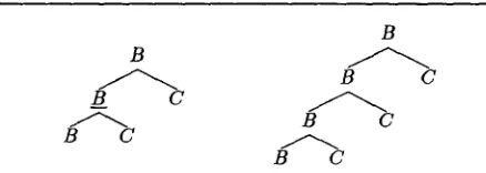
if (i) p is not the root of Q; and (ii) S matches Q at the root node. It is easy to see t h a t the fact t h a t lhs(r) has some periodic node is a necessary condition for r to be critical. Let the root of S be the i-th child of a node n / in Q, and let Qc be a c o p y o f Q . We write Qp to denote the tree obtained starting from Q by excising S and by letting the root of Qc be the new i-th child of

hi.

Finally, call nl the root of Qp and n2 the root of Q. E x a m p l e 5 Figure 6 depicts trees Q and Qp. T h e periodic node p of Q under consideration is indicated by underlying its label. []

Let us assume t h a t rule r is critical and t h a t p is the only periodic node in Q. We add Qp to set lhs(R) and construct AG accordingly. Algorithm 1 should then be modified as follows. We call

p-chain

any sequence of one or more subtrees of C, all matched by Q, t h a t partially overlap in C. Let n be a node of C and let q =

state(n).

Assume t h a t n2 E q and call S the subtree of C at n m a t c h e d by Q (S exists by L e m m a 1). We distinguish two possible cases. Case 1: If nl E q, then we know t h a t Q also matches some portion of C t h a t overlaps with S (at the node m a t c h e d by the periodic node p of Q). In this case S belongs to a p-chain consisting of at least two subtrees and S is not the b o t t o m - m o s t subtree in the p-chain.

Case 2: If nt ~ q, then we know t h a t S is the b o t t o m - m o s t subtree in a p-chain.

Let i be the index of rule r under consideration. We use an additional set

chain(i).

Each node n

of C such t h a t

n~ 6 state(n)

is then inserted in

chain(i)

if

state(n)

satisfies Case 1 above, and is inserted in

rule(i)

otherwise. Note t h a t

chain(i)

is n o n - e m p t y only in case

rule(i)

is such. Whenever i is retrieved from H , we process each node n in

rule(i),

as usual. But when we u p d a t e our d a t a structures with the procedure

update,

we also look for match- ings of lhs(ri) at nodes of C in

chain(i).

T h e overall effect of this is t h a t each p-chain is considered in a b o t t o m - u p fashion in the application of r. This is compatible with the post-order application require- ment.

T h e above technique can be applied for each periodic node in a critical rule, and for each critical rule of G. This only affects the size of

AG,

not the t i m e requirements of Algorithm 1. In fact, the proposed preprocessing can at worst double

ha.

5 D i s c u s s i o n

In this section we relate our work with the existing literature and further discuss our result.

There are several alternative ways in which one could see transformation-based rewriting systems. T T S ' s are closely related to a class of g r a p h rewr.iting systems called neighbourhood-controlled embedding graph g r a m m a r s (N CE g r a m m a r s ; see (J anssens and Rozenberg, 1982)). In fact our definition of the relation and of the underlying [/] o p e r a t o r has been inspired by similar definitions in the N C E formalism. A p a r t from the restriction to tree rewriting, the main difference between N C E g r a m m a r s and T T S ' s is t h a t in the latter formalism the productions are totally ordered, therefore there is no recursion.

Ordered trees can also be seen as ground terms. If we extend the alphabet ~ with variable symbols, we can redefine the ~ relation through variable sub- stitution. In this way a T T S becomes a particular kind of term-rewriting system. T h e idea of imposing a total order on the rules of a term-rewriting system can be found in the literature, but in these cases all rules are reconsidered for application at each step in the rewriting, using their priority (see for instance the priority term-rewriting systems (Baeten, Bergstra, and Klop, 1987)). Therefore these systems allow recursion. There are cases in which a critical rule in a T T S does not give rise to order-dependency in rewriting. Methods for deciding the confluency property for a term-rewriting system with critical pairs (see (Dershowitz and J o u a n n a u d , 1990) for definitions and an overview) can also be used to detect the above cases for T T S .

As already pointed out, the translation p r o b l e m investigated here is closely related with the standard tree p a t t e r n matching problem. Our a u t o m a t a

[image:7.612.59.278.204.282.2]

(8)

(our set lhs(R)) requiring an amount of space which is exponential in the degree of the pattern trees, as an improvement, our transition function does not de- pend on this parameter. However, in the worst case the space requirements of both algorithm are exponential in the number of nodes in lhs(R) (see the analysis in (Hoffmann and O'Donnell, 1982)). As already discussed in Section 3, the worst case condition is hardly met in natural language applications. Polynomial space requirements can be guaranteed if one switches to top-down tree pattern matching algorithms. One such a method is reported in (Hoff- mann and O'Donnell, 1982), but in this case the running-time of Algorithm 1 cannot be maintained. Faster top-down matching algorithms have been reported in (Kosaraju, 1989) and (Dubiner, Galil, and Magen, 1994), but these methods seems impractical, due to very large hidden constants.

A tree-based extension of the very fast algorithm described in (Roche and Schabes, 1995) is in prin- ciple possible for transformation-based parsing, but is likely to result in huge space requirements and seems impractical. The algorithm presented here might then be a good compromise between fast parsing and reasonable space requirements.

When restricted to monadic trees, our automaton Ac comes down to the finite state device used in the well-known string pattern matching algorithm of Aho and Corasick (see (Aho and Corasick, 1975)), requiring linear space only. If space requirements are of primary importance or when the rule set is very large, our method can then be considered for string- based transformation rewriting as an alternative to the already mentioned method in (Roche and Sch- abes, 1995), which is faster but has more onerous space requirements.

A c k n o w l e d g e m e n t s

The present research was done while the first author was visiting the Center for Language and Speech Processing, Johns Hopkins University, Baltimore, MD. The second author is also a member of the Cen- ter for Language and Speech Processing. This work was funded in part by NSF grant IRI-9502312. The authors are indebted with Alberto Apostolico, Rao Kosaraju, Fernando Pereira and Murat Saraclar for technical discussions on topics related to this paper. The authors whish to thank an anonymous referee for having pointed out important connections between TTS and term-rewriting systems.

R e f e r e n c e s

Aho, A. V. and M. Corasick. 1 9 7 5 . Efficient string matching: An aid to bibliographic search. Communications of the Association for Comput- ing Machinery, 18(6):333-340.

Baeten, J., J. Bergstra, and 3. Klop. 1987. Prior- ity rewrite systems. In Proc. Second International Conference on Rewriting Techniques and Applica- tions, LNCS 256, pages 83-94, Berlin, Germany. Springer-Verlag.

Brill, E. 1993. Automatic grammar induction and parsing free text: A transformation-based approach. In Proceedings of the 31st Meeting of the Association of Computational Linguistics, Colum- bus, Oh.

Brill, E. 1995. Transformation-based error-driven learning and natural language processing: A case study in part of speech tagging. Computational Linguistics.

Brill, E, and P. Resnik. 1994. A transformation- based approach to prepositional phrase attach- ment disambiguation. In Proceedings of the Fifteenth International Conference on Computa- tional Linguistics (COLING-199~), Kyoto, Japan. Chomsky, N. 1965. Aspects of the Theory of Syntax.

The MIT Press, Cambridge, MA.

Chomsky, N. and M. Halle. 1968. The Sound Pat- tern of English. Harper and Row.

Cormen, T. H., C. E. Leiserson, and R. L. Rivest. 1990. Introduction to Algorithms. The MIT Press, Cambridge, MA.

Dershowitz, N. and J. Jouannaud. 1990. Rewrite systems. In J. Van Leeuwen, editor, Handbook of Theoretical Computer Science, volume B. Else- vier and The MIT Press, Amsterdam, The Nether- lands and Cambridge, MA, chapter 6, pages 243- 320.

Dubiner, M., Z. Galil, and E. Magen. 1994. Faster tree pattern matching. Journal of the Association for Computing Machinery, 41(2):205-213.

Hoffmann, C. M. and M. J. O'Donnell. 1982. Pat- tern matching in trees. Journal of the Association for Computing Machinery, 29(1):68-95.

Janssens, D. and G. Rozenberg. 1982. Graph gram- mars with neighbourhood-controlled embedding.

Theoretical Computer Science, 21:55-74.

Kaplan, R. M. and M. Kay. 1994. Regular models of phonological rule sistems. Computational Lin- guistics, 20(3):331-378.

Kosaraju, S. R. 1989. Efficient tree-pattern matching. In Proceedings of the 30 Conference on Foun- dations of Computer Science (FOCS), pages 178- 183.

Roche, E. and Y. Schabes. 1995. Deterministic part of speech tagging with finite state transducers.

Computational Linguistics.