Munich Personal RePEc Archive
Optimizing the Structure of Mongolian
Foreign Trade and the Alternative Policy
of Successful Transition
Byambasuren, Tsenguunjav and Gochoo, Munkh-Erdene
Bank of Mongolia, Institute of Finance and Economics
2 February 2015
Online at
https://mpra.ub.uni-muenchen.de/61803/
Optimizing the Structure of Mongolian Foreign Trade and the
Alternative Policy of Successful Transition
Tsenguunjav Byambasuren†
Bank of Mongolia
Munkh-Erdene Gochoo‡
Institute of Finance and Economics
February 2, 2015
Abstract
This paper aims to make an alternative development policy which can encourage the foreign trade efficiency. In order to make the policy, the current situation of Mongolian Foreign Trade has been determined and invented the product sectors that have a chance to be developed for the further. In this paper, several methods such as Revealed Comparative Advantage (RCA) method, Product Space Analysis or Monkey and Tree Model, Opportunity Index, and Gravity Model have been used to make analysis. The paper illustrates that firstly, Mongolian Foreign Trade has been becoming more dependent from a single country, a single product and there is no structural shift. In other words, the most part of Mongolian export goods consist of the products that have low sophistication level and low value added, and based on natural resources. Also, the diversification of export goods basket is poor and even no unique products are included in the basket. Therefore, this paper suggests an alternative development policy based on Hidalgo, Ricardo Hausmann, and Bailey Klinger’s policy recommendations and foreign trade policy experience of China whose economic performance was the best in the world last 30 years.
JEL Classification Numbers: C55, F14, F42
Keywords:Revealed Comparative Advantage (RCA), Product space model, Structural transformation
†
International Economics Department, Bank of Mongolia. E-mail: tsenguunjav.b@gmail.com.
‡
1
Introduction
Adam Smith regards industrialization and foreign trade as a mean of that a state turns into wealth and distributes it to its people at the Wealth of Nations. According to the concept, wealthy and abundant life belongs not only to aristocrats but also it may be created by typical people via labor and efforts. Thereon, Jan Batist Sei and Fredrick Bastia have noticed benefits of industrialization as that “it assists human named animal to achieve real human characteristics” and determined that it is the most optimal mean that trade of made products to other countries creates wealth by human labor. Thus, all of above show that industrialization and foreign trade are resources of wealth (Scausen, 2010).
In contemporary economy, the concept “Foreign trade” has been changed into very essential question during last 60 years. There have been cases that growth of foreign trade of some countries has exceeded over that of GDP. However a policy which replaces import was been widely applied during 1950-1970, the result of export oriented policy of Asian tiger countries was weak. But, other countries could make substantial changes in short-term by implementing export-oriented policy.
Improbity and corruption spilled out of control and ineffective resource distribution were been seen during the period when pursued to develop domestic market by importation protectionism before 1980. The consequence demonstrates that the policy couldn’t achieve its goal. Rather, countries have been guided by free trade policy which directs to exportation and aimed to ensure economic growth by creating competency since 1980. This policy has been extremely effective and played an important role to make changes in international foreign trade structure.
During last 20 years, great ambition of countries to earn benefits from the foreign trade has led to adoption of treaties such as free zone and free trade agreements and active unity of countries in the world. The year 1994 was the unification epoch. 124 countries joined in Uruguay treaty, touched upon issues on intellectual property and intended to establishment of a new institution.
However, General agreement of tariff and tax failed at first, it was backbone of World Trade Organization. Almost half of countries in the world including leaders of Bulgaria, The Indonesia, and Asia-Pacific countries have set a goal that industrialized countries have developed perfect free trade by 2010 and developing countries have developed it by 2020. Like this, globalization is intensifying and trade is being released constantly.
It considers that foreign trade structure of particular country reflects its economic structure. In other words, export goods sectors have well developed and import good sectors have underdeveloped in domestic industrialization. On the other hand, the country exports goods made by lesser expenses and imports goods that can’t be made itself. This is the Revealed comparative advantage’s principle.
of profits gained from mining. If not, a question “what will produce?” will arise seriously after minerals come to end.
This paper intends to determine a “possible development option” by evaluating current Mongolian potentiality, nominating sectors which have ability to grow up in short term based on the evaluation and recommending most rational forms and levels of government’s interference in development of these sectors. Benefits and originality of this paper is resides in discovering a possible option that can separate from dependency by turning Mongolia to producer country, its economy is stable and under the immunity, its people are wealthy and rich, have great income and decrease gap between rich and poor.
The paper consists of Conditional analysis and Policy analysis. Conditional analysis
contains: (i) Evaluation of Mongolian foreign trade structure, its dependency, concentration,
gravitation of trade partners and determination of sectors that produces goods which have
potential to expand. (ii) Evaluation of manufacturing level and corporative advantages of
Mongolian export goods, outline of product space and determination products which have capacity to develop.
Methodologies such as Gravity model of foreign trade developed by Timbergen and Poyhonen, indexes which value foreign trade concentration and dependency, Revealed Comparative Advantages method which evaluate products’ comparative advantage developed by Balassa and Products’ space analysis developed by Hidalgo, Haussmann, Klinger and Baraboso and Index of opportunity developed by Jesus Felipe, Utsav Kumar and Arnelyn Abdon have been applied in orther to carry out an analysis. In frame of policy analysis, most optimal interference level of government which is effective in increasing export of value-added goods in foreign trade and growing benefits of foreign trade based on current situation has studied by associating with Chinese foreign trade policy and recommendation of policy developed by Ricardo, Haussmann, Klinger and Hidalgo.
2
Literature Review
2.1
Necessity of General Theory of Foreign Trade Policy
Comparative study on various countries which developed by McGovan and Shapiro seems that it has generally eliminated weakness that lack of prime theory of foreign trade and has demonstrated treats lack of prime theory of foreign trade. The lack of foundational theory in this sector leads several serious consequences. For instance:
• We have unable to explain relations of findings in particular sector and can
recommend only a hypothesis on behavior of foreign trade;
• We might hope for only luck in order to gain hypothesis of an effective work;
• The work is temporary, unplanned, without required reason to select particular case,
non-systematic and inconstant; and
Structure of Foreign policy theory is needed to investigate daily interaction in international relations and compare particular foreign policy. Also, structure of the theory which devoted to analyze foreign policy is not only issue which is relevant to universities. That is a political issue in connection with increasingly raising level of correlation between countries and unification of global interests. Wide range of data base with empiric study and data attracted attention of specialists who work out the structure of Foreign policy general theory. Scientists have concluded its evolutionary dispersion in taking advantage of many methods:
• Collation of particular condition compared with given country’s behavior with
empiric studies;
• Analysis which gives substantial weight to foreign policy process and factors that
influence in foreign policy;
• Scientific methods and models which are devoted to foreign policy analysis such as
correlation, national and public models; and
• Studies which are strive to provide global model.
2.2
Foreign Trade Policy of Developing Countries
Since WWII, building and creation of industrial sector which was the key of economic development has greatly influenced in trade policy of most developing countries and the best and most successful mode was protection of domestic producers form international competence during 30 years.
Import-substituting Industrialization: In order to foster their domestic industrial sectors, developing countries have tried to accelerate their development by curbing imports of industrial products from WWII to 1970. This strategy has been exercised widely.
Figure 2-1. Tariff level of the countries, 1980-1998
Source: National Statistical Office
Industrialized countries have reached the peak of protectionism in 1930s. In 1947, General Agreement Tariff and Tax was established and began weakening the protectionism. Tariff which was 50% in 1940s decreased to 41% on an average by 1988.
0 10 20 30 40 50 60 70
ӨмнөдАзи ЛатинАмерик ЗүүнАзи ДэдСахарын Африк
ДундадЗүүнба ХойдАфрик
ЕвропбаТөвАзи Ажүйлдвэржсэн орнууд
1980-85 1986-90 1991-95 1996-98
Southern Asia
Latin America
Eastern Asia
Sub-Saharan Africa
Northern Africa
EU & Central Asia
There were lots of negative consequences like businessmen who were at the rule of a state took trade power their hands and created inappropriate distribution of resource and corruption spread because the state provide quota and licenses as tariff and non-tariff means. But, the import-substituting policy has been abolished from 1980 and initialization of implementing export-oriented policy has completely changed foreign trade type of developing countries.
Trade liberalization since 1985: In the middle of 1980s, some of the developing countries have changed tax to lower level and eradicated importation quota, other restrictions and barriers in trade. The transition of developing countries to more liberal trade and commerce was one of the marked events in trade policy in last two decade.
Since 1985, many countries have declined customs duty and abolished importation quota and opened their economy for import competence in general. Table 2-1 shows foreign policy trend of India and Brazil which have chosen importation substitute as their development strategy. Both of them had industrial sectors which were highly protected in 1985.
South-East Asian miracle of export-oriented industrialization: Developing countries united with the concept that there was opportunity to create industrial foundation by replacing imports with domestic industrial products in 1950s and 1960s. But, it has been seen that there are other potential way to support industrialization since 1960s: Export of industrial products to developed countries. Likewise, the World Bank names countries which have developed by this model as High-performing Asian economies: some economies of them had over 10% of annual growth. From the middle of 1960s to Asian crisis, GDP of “Tiger” countries grew up by 8-9% on an average.
[image:6.595.161.435.556.617.2]However, that of USA and Western European countries increased by 2-3% at the same time. The recent growth of Asian other economies has reached level that can compare with them and China’s economic growth level is over 10%. Besides the high level of growth, High-performing Asian economies have another specific feature: They are open to international trade. Indeed, rapidly growing Asian economies are more export-oriented than other developing countries in particular Latin America and South Asia (Krugman & Obstfeld, 2007).
Table 2-1. Protectionism Impact in industrial sectors
India Brazil
1980s 126 77
1990s 40 19
Source: Krugman & Obstfeld (2007)
this model as High-performing Asian economies-some economies of them had over 10% of annual growth.
From the middle of 1960s to Asian crisis, GDP of “Tiger” countries grew up by 8-9% on an average. However, that of USA and Western European countries increased by 2-3% at the same time. The recent growth of Asian other economies has reached level that can compare with them and China’s economic growth level is over 10%. Besides the high level of growth, High-performing Asian economies have another specific feature: They are open to international trade. Indeed, rapidly growing Asian economies are more export-oriented than other developing countries in particular Latin America and South Asia (Krugman & Obstfeld, 2007).
Trade policy of High-performing Asian economies: Most economists believe that economic high ratio is a reason for success of economy. For example, both of import and export of Thailand jumped in 1990s. Why? Its reason was that the country was destination which was favorable for sophistication of Multinational corporations. These corporations directly produced most of its new export and import of raw materials for their sophistication turned into a large wave in its import capacity. In such a manner, Thailand gained a large amount of export and import.
Industrialization policy of High-performing Asian economies: Some analysts rely on that efficiency of free trade policy has generated accomplishment of the High-performing Asian economies. In practice, majority of countries which their economy achieved growth pursued more comprehensive industrial policy such as not only restriction on customs duty and import and export subsidy but also lower interest of loan and promotion of government for research and examination. In general, it is difficult to evaluate industrial policy. Studies on the issue were arguable and problematic because of 3 reasons.
Firstly, high-performing Asian economies followed variety of policy: Whilst almost free
policy was exercised in Hong-Kong, economy of Singapore was guided and regulated by its
government accurate direction.South Korea has enhanced structure of their larger industries
in step by step and small household enterprises are still dominating in economy of Taiwan. The all economies couldn’t reach the same level of growth yet.
Secondly, if the industrial policy had not come into the limelight, its actual impact in industrial structure might not have been such a substantial. World Bank noted that only surprisingly little proof of the countries with concrete industrial rapidly fostered, not seen before, industrial sector at study on Asian miracle.
Finally, the industrial policy of most successful economies had several mistakes. For instance, South Korea was guided by a policy to develop heavy industrial and chemical sectors such as chemicals, steel and automobiles. This policy affirmed that it had spent a large amount of expenses and it was considered as an improper policy and refused. Maybe, the industrial policy was not a key of Asian economic growth (Krugman & Obstfeld, 2007).
2.3
Trend of International Trade and Integration
covered wide range of activities. But, the objective didn’t realize because of USA Congress’ disapproval. However, the International trade organization remained under the name of General agreement of Tariff and Tax. The agreement, adopted in 1947, has been passing through 8 phases up to now in total. Please find the phases in Table 2-2.
Table 2-2. Rounds of GATT
Country Beginning
date Duration
Number of
states Topic Results
Geneva April, 1947 7 months 23 Tariff Adopted GATT and
negotiated, 45,000 tariffs
Annecy April, 1949 5 months 13 Tariff Negotiated 5,000 tariffs
Torg September,
1950 8 months 38 Tariff
Negotiation on 8,700 tariffs
Geneva II January,
1956 5 months 26
Tariff and Japanese permition
Tariff rebare, $2.5 billion
Dillon September, 1960
11
months 26 Tariff
Tariff rebare, $4.9 billion
Kennedy May, 1964 37
months 62
Tariff and agains
dumping Tariff rebate $40 billion
Tokyo September,
1973
74
months 102
Measuremnet of tariff and non-tariff
Evaluation of tariff rebate, beyond $300 billion
Uruguay September, 1986
87
months 123
Tariffic and non-tarific measures, charter, service, intellectual property riths, agriculture and WTO
Establsihed WTO and expanded its activities and tariff was reduced by 40%
Doha September,
2001 - 141
Tariffic and non-tarific measures, agriculture, labor standard, invironment, competitiveness, investment, patent etc
-Developing countries have confronted with two issues. One is an issue on improvement of legal environment and another one is an issue on establishment of customs rate, government procurement, product standard and measures against dumping (Martin, Trade Policies, Developing Countries, and Globalization, 2001).
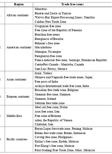
Table 2-3. International free-zones
Region Trade free-zones
1. African continent
Mauritius
Bizerte and Zarzis in Tunisia
Walwis Bay Export Processing Zones, Namibia Calabar Free Trade Zone
2. American continent
Uruguayan free zone
Free Zone of the Republic of Panama Brazilian free-zones
Baraguassu of Brazilia Bahama’s free zone Macuiladoras Managua, Nicaragua Paraguayan free zone
Franca industial free zone, Santiago, Dominican Republic CentrePort Canada - Manitoba, Canada
Sant Luis Potocy, Mexico
3. Asian continent
Izmir, Turkey
Okinava and Nagasaki free trade zones, Japan Free posts of India
Arshiya-International trade free zone, India
4. Eurpean continent
Bruselian free trade zone, Belgium Shannon free zone, Shannon Shannon, Ireland
Sebirian free trade zone
5. Middle-East
Jebel Ali free zone, Dubai Aras free zone, Iran Free zone of Bahrain
Aden, the Republic of Yemen Chabahar, Iran
6. Pacific countries
Bayan Lepas free trade zone, Penang, Malasia Batam free trade zone, Batam, Indonesia Caviteg free zone, Philippines
Kulim’s free zone, Kedah, Malasia Port Klang’s free zone, Malasia
Pasir Gudang Free Trade Zone, Johor, Malaysia
Source: National Development Institution
Table 2-4. Regional integration blocks
Scope Blocks Countries within the block
1.
Industrialized countries and developing countries
European Union /EU/ Belgium, France, Germany, Italy,
Neiderland, Denmark, Great Britain, Greece
European economic zone Island, Liechtenstein, Norway
The Euro-Meditarranean free
trade economic zone EU -Tunisia, EU-Marraco
Bilateral agreements between EU and East European countries
Hungery, Poland, Bulgaria, Romania Estonia, Latvia, EU-Lithuania, EU-Czech, EU-Slovakia Canada-The United States free
tarde zone Canada- USA
North American Free Trade
/NAFTA/ Canada, USA. Mexico
Asian Pacific Economic Cooperation /APEC/
Brunei Darussalam, Canada, Indonesia, Malaysia, Newzealand, Singapore etc Organization of Economic
Cooperation and Development
Ausralia, Canada, Czech, Denmark, France, Germany, Italy, Japan, South Korea Organization of the Petroleum
Exporting Countries /OPEC/
Iran, Iraq, Kuwait, Saudi-Arab, Venezuela, Qatar, Nigeria, Indonesia , Libya, Ageria
2. South America and Caribbean
Andean Pact Bolivia, Columbia, Equador, Peru, Venezuela
The Central American Common Market /CACM/
El Salvador, Guatemala, Hoduras, Nicaragua, Costa Rica
Southern Common Market
South America /MERCOSUR/ Argentina, Brazilia, Paragua, Urugua
Group of Tree Columbia, Mexico, Venezuela
Latin American Integration Association /LAIA/
Mexico, Ergentina, Bolivia, Brazilia, Chile, Columbia, Equador, Paragua, Urugua, and Venezuela
Caribbean Community and Common Market /CARICOM/
Antigua and Barbuda, Barbados, Jamaica, St. Christopher and Nevis , Trinidad and Tobago, Belize, Dominica, Grenada
3. Sub-Saharan Africa
Cross-Border Initiatives Brundi, Comoros, Kenya, Madagascar, Rwanda, Swaziland, Tanzania, Uganda East African Cooperation Kenya, Tanzania, Uganda
Central African Finance and Economic Association
Cameroon, Republic of Central Africa, Chad, Congo, Gabon, Equatorial Guinea
The Economic Community of West African States
/ECOWAS/
Benin, Burkina Faso, Kape-Verde, Cote d’Ivore, Gambia, Gana, Guinea, Mali, Nigeria, Togo
Common Market for Easter and Southern Africa
Angola, Brundi, Comoros, Egipty, Ethiopia, Kenyam Lesoto, Malawi, Mauritius
Souther African Development Community /SADC/
Botswana, Malawi, Tanzania, Zimbabwe, Namibia, Pepublic of South Africa, Mauritus
Table 2-4. Regional integration blocks (continued)
Scope Blocks Countries within the block
3. Sub-Saharan Africa
West African Economic and Monetary Union
Benin, Burkina Faso, Cote d’Ivoire,
Maurintania, Nigeria, Senegal, Togo, Guinea-Bissau
South African Custom Union /SACU/
Botswana, Lesotho, Namibia, Republic of South Africa, Swaziland
Economic Association of
Great Lakes Region Brundi, Rwanda, Congo
4. Middle-East and Asia
Association of South East Asian Nations /ASEAN/
Indonesia, Malaysia, Philippines, Singapore, Thailand, Vietnam, Myanmar, Lao PDR, Cambodia
ASEAN+3 Japan, China, South Korea
Shanghain Cooperation Organization /SCO/
China, Russia, Kazakhstan, Kyrkyz, Tajikstan, Uzbekistan
Central Asian Regional Economic Cooperation /CAREC/
Afganistan, Azerbaijan, China, Kazakhstan, Kyrgyz, Mongolia, Tajikstan, Uzbekistan
Culf Cooperation Council /GCC/
Bahrain, Kuwait, Oman, Qatar, Butan, India, Moldavian, Nepal, Pakistan, Shri-Lanka
Source: National Development Institution
Trade interconnection among regions reduces in barriers in trade and makes more efficient trade.
Economic outcome of regional integrations and issues on expenses: Membership in regional integration agreements causes negative and positive effect in almost every sector of its economy. Whilst some sectors are opened to an opportunity of expansion, some of them shrinks and tightens due to competence, scale effect and influence of trade and location. The influence of competence and scale effect will increasingly integrate economy of particular country in united markets. The larger market will encourage scale effect and firm producers and sophisticationrs of member states with mutual competence.
Also, it may be made changes in import price of suppliers, scale of market, competence as well as tendency of foreign investment attraction of non-member states. Regional integration intensifies competence within only the block as well as enhances competence of foreign companies which export their products to the integrated market. Several activities carry out during the integration process such as convergence, clustering and divergence and the activity may efficient and inefficient to particular country depending on its condition and circumstance.
Location influence can change actual profit of consumer and producers and income which is generated from tax.
The trade diversion and trade creation may emerge at each type of integrations. The free-trade zone may form the free-trade diversion in pattern that transfers the free-trade from more efficient suppliers which are out the free-trade zone to more inefficient supplier which are within the zone. The trade creation means new creation of trade structure and classification which have been missed in the zone. In other words, supply will run up at the result of producers’ efficient operation gaining profits.
2.4
Review on Empirical Analysis
2.4.1 The Gravity Model
For the beginning, there were a few theoretical evidences in this field and this situation has disappeared since the second part of 1970s. Anderson (1979) attempted to redevelop the Gravity model based on goods’ discrimination. Bergstrand (1985, 1989) proposed the bipartite trade theoretical models that used Gravity model equations as simple monopolistic competition model by the studies. Finally, Deardoff (1995) proved that Gravity model equations can define many models and it can be explained by standard trade theories (Martinez-Zarzoso & Nowak-Lehmann, 2003).
Many studies have tended to develop the Gravity model equations. Some of them associated with these articles. Matyas (1997, 1998), Chen and Wall (1999), Breuss and Egger (1999) and Egger (2000) developed econometric definition of the Gravity model equations. Then, Bergstrand (1985), Helpman (1987), Wei (1996), Soloaga and Winters (1999), Limao
and Venables (1999) and Bougheas et al (1999) upgraded the factors that considered in the
model and added some new factors (Martinez-Zarzoso, 2003).
Timbergen (1962) and Poyhonen (1963) implemented TheGravity Model to international
trade flow for the first time. Hence, researchers started to use this model wide spread for their articles. Furthermore, studies such as population movements and foreign investment were
implemented widely. This model includes the dummies that determined exports of country 𝑗
from country 𝑖, their GDPs, population and distance between them (Martinez-Zarzoso, 2003).
Inmaculada Martinez-Zarzoso studied bipartite trade flow for European Union (EU), North American Free Trade Agreement (NAFTA), Carribbean Community, Centro-American Common Market and Mediterranean Countries etc. He evaluated gravity equations by using Least Square method and Panel data of total 47 countries from 1980 to 1999.
Inmaculada Martinez-Zarzoso and Felicitas Nowak-Lehmann (2002) evaluated the gravity model between Mercosur-European Union and purposed to calculate effects of their recent trade agreement. Their work based on the panel data analysis of 4 official members of
Mercosur included Chile and 15 countries of EU. They used Extended Gravity model. This
model includes infrastructure, GPD per capita of 𝑖 and 𝑗 countries and real exchange rate
more than its traditional model. As a result of this work, income sensitivity was close to its theoretical value and population of exporting country effect was negative. All factors that added to this model were statistical significant, although, the factor of importing country’s infrastructure wasn’t statistical significant.
2.4.2 Revealed comparative advantages
Balassa (1965) developed the concept of revealed comparative advantage, which is the measure of the share of a given product in a country’s total exports relative to the product’s share in total world exports, that is, a ratio of relative export structure. If one finds, for example, that the RCA of a country is high for a commodity group requiring the intensive use of capital, one can conclude that the country has a relatively large endowment of capital.
Kang-Taeg Lim (1997) studied the foreign trade of Democratic People’s Republic of Korea (DPRK) by using Comparative Advantage model and database between 1970 and 1992. The result of study showed that foreign trade products of DPRK are being modified from Ricardo’s goods to Heckscher-Ohlin’s goods. The consumer goods export of DPRK is centralized on the Communist market and production goods import relies on the source of non-Communist market. In conclusion, DPRK is working for developing its economic structure, main structure of goods is moving to goods that use standard technology from the goods that uses natural resources, furthermore, they have a chance to produce goods that use advanced technology.
2.4.3 Product space and structural revolution
A study of Ricardo Hausmann (2006) and Bailey Klinger (2006) is one of the studies on the issue. They have initially developed the concept of product space. According to their study, think of a product as a tree and the set of all products as a forest. The monkey jumps from one tree to another and if the tree is distant, monkey can’t jump to it. Distance of trees demonstrates that there is possibility to produce new products based on present potential resources. Also, government is able to bring close the trees by implementing suitable policy. For instance, if infrastructure, electricity and water supply are solved by establishment of free-zone, there will be more opportunity to produce new products there. Structural revolution of the product space and acceleration of conversion depend on how distant new product space.
impact within their sector will be created by firms if a country advanced comparative advantage of a particular product. But, inter-sector indirect impact will be created if the potential opportunities reduce their space in between the product.
Ricardo Hausmann (2007) and Bailey Klinger (2007) have done a comparative study of Chilean structural transformation with other countries using data between 1960 and 2007. However Chile could create large amount of increase in its export service, it has limited space to expand export market, lesser degree of export sophistication, product space without connection and fewer opportunities to do structural transition in the future.
Furthermore, its present condition is ordinary but there may be risk make trouble in further. Basic prize of its export products lacks of growth and is dropping in compared with other countries. For the current export structure, there are not near trees. Due to distant space among trees, there is high possibility that the jump will fail.
It is necessary to find product space because missing opportunities to enhance its product quality in some ways. Base on international experience, this effort is issue of public policy and government needs to take policy measures. For instance, establishment of special zone and attraction of foreign investment. State policy should direct to create new market not to improve now existing sectors.
Ricardo Hausmann (2009) and Bailey Klinger (2009) worked on structural revolution of Caribbean countries. Emphasizes government policy is valuable. Experts have identified potential ways and means of government measures.
Jesus Felipe, Utsav Kumar and Arnelyn Abdon (2010) have developed a new Index of Opportunity. The index consists of 4 indexes such as:
• Sophistication index;
• Diversification index;
• Standardness index;
• Open forest measurement
as measure of the potential for further structural change. It allows determining a country’s capabilities to undergo structural transition though the index.
Their study results suggest that China, Brasilia, German, India and the Indonesia have accumulated a significant number of capabilities. But, Russian Federation has shown lower index of opportunity. China whit lower income acquires most advantages or comparative advantages of 265 products whilst the Russian Federation owns the lowest advantage or advantages of only 105 products.
well in the long run. It is important to diversify and increase the level of sophistication of
their export baskets in order to do so. These countries have inseminated in plentiful and
productive soil and have opportunity to harvest substantial amount of crops if it will be sustained by right policy. For other countries, situation is worse.
3
Methodology and Data
Foreign trade is study through its flows analysis and its structural transition analysis. This paper evaluates foreign trade flows using the gravity model.
3.1
The Gravity Model
The model was derived from universal law of gravity by Tinbergen. Universal gravity correlates directly with weight of particular two planets and conversely with space between planets. This imagination is applied so that gravity is to be as export, weight of planets is to be as GDP and space between planets is to be geological locations of two countries.
Traditional gravity model:
𝑋!" =𝛽!𝑌!
!!
𝑌!
!!
𝐷!"!!𝐴!"!!𝑢 !" (3-1)
where:
𝑌! - GDP of exporting country;
𝑌! - GDP of importing country;
𝐷!" - distance between capitals of two countries;
𝐴!" - coefficient of other factors;
𝑢!" - regression residual.
Expanded gravity model:
𝑋!" =𝛽!𝑌!
!!
𝑌!
!!
𝑁!
!!
𝑁!
!!
𝐷!"!!𝐴!" !!
𝑢 !" (3-2)
where:
𝑌! 𝑌! - GDP of exporting and importing countries;
𝑁! 𝑁! - populations of exporting and importing countries;
𝐷!" - distance between capitals of two countries;
𝐴!" - coefficient of other factors;
𝑢!" - regression residual.
Another version of the model indicated GDP per capita instead of population:
𝑋!" =𝛾!𝑌!
!!
𝑌! !!
𝑌𝐻!!!𝑌𝐻!
!!
𝐷!"!!𝐴!" !!
𝑢!" (3-3)
where:
𝑌𝐻! 𝑌𝐻! - GDP per capita of expotring and importing countries.
𝛽! = −𝛾!
𝛽! = −𝛾!
𝛽! =𝛾!+𝛾!
𝛽! = 𝛾! +𝛾 !
(3-4)
Berstrand (2000) has noted that it is suitable to use the second equation to analyze export of a particular special product. But, Endoh (2000) considered that it is appropriate to apply the first equation to evaluate total export.
A high level of income in the exporting country indicates a high level of production, which increases the availability of goods for export.
Therefore 𝛽! is expected to be positive. The coefficient of 𝑌!, 𝛽! is also expected to be
positive since a high level of income in the importing country suggests higher imports. The coefficient estimate for population of the exporters, 𝛽!, may be negatively or positively
signed (Oguledo and Macphee, 1994), depending on whether the country exports less when it
is big (absorption effect) or whether a big country exports more than a small country
(economies of scale). The coefficient of the importer population, 𝛽!, also has an ambiguous
sign, for similar reasons. The distance coefficient is expected to be negative since it is a proxy
of all possible trade costs (Martinez-Zarzoso, 2003).
3.2
Revealed Comparative Advantages (RCAs)
The main basis of the theory of international specialization has been the principle of comparative advantage, although the principle now goes far beyond the original explanation provided by Ricardo. The concepts of comparative advantage and competitiveness are often confused with one other. Those are, however, quite different in reality. When instability in exchange rates produce disequilibria, competitiveness is seriously disturbed and any analysis based on it is highly inadequate. Therefore any explanation of international specification increasingly has to take into account some measure of comparative advantages. In this case, the comparative advantages concerned are those that are revealed by the results of international trade.
Balassa (1965) developed the concept of revealed comparative advantage, which is the measure of the share of a given product in a country’s total exports relative to the product’s share in total world exports, that is, a ratio of relative export structure. In line with Balassa s suggestion, revealed comparative advantage (RCA) has taken two forms as follows:
Net exports as a portion of total trade in a commodity group:
𝑥!" = 𝑋!" −𝑀!" 𝑋!" +𝑀!" (3-5)
𝑋 and 𝑀 stand for the value of exports and imports respectively, 𝑖 denotes a commodity
The measure ranges between 1 (corresponding to no exports by country 𝑗 in commodity group 𝑖) and 1 (corresponding to no imports for country 𝑗 in commodity group 𝑖). Even
though the interpretation of this measure is subject to criticism, because imports are influenced by the system of protection used in a country, this measure has some merit: (a) it shows the significance of net flows in any commodity group; (b) its absolute value 𝑥!"
represents the portion of inter-industry trade in the total trade of the concerned commodity
group 1− 𝑥!" is the corresponding portion of intra-industry trade).
Theoretically, this measurement is used widely spread and we choose the following form for the empirical study:
𝑅𝐶𝐴!
,!" = 𝑋!" 𝑋!" !
!!!
𝑋!" !
!!!
𝑥!"
!
!!! !
!!!
(3-6)
The indicators 𝑥!" and 𝑚!" may have opposite directions. A priori, comparative advantage must meet the conditions, 𝑥!" > 1 and 𝑚!" < 1, while comparative disadvantage requires
𝑥!" < 1 and 𝑚!" > 1. One could, however, encounter the case that 𝑥!" > 1 and 𝑚!" >1, or
𝑥!" < 1 and 𝑚!" <1. How can one make a conclusion about comparative advantage in those
cases? As an attempt to overcome this ambiguity, we can consider Equation (3-‐1), (3-‐2), and
(3-‐3).
Lafay (1992) and Murrell (1990) agree that the trade balance is more likely to be well-behaved than the exports side or imports side only. Since the world average of trade balance will be zero, one cannot define any statistic of the trade balance as exactly analogous to
Equation (3-‐2) and (3-‐3). As Murrell (1990) suggested, therefore, the ‘net’ trade
performance in a commodity which is still useful as a descriptive measure with a natural scale will be examined. According to Murrell (1990), one can define.
𝑋!" is the amount of exports of a commodity 𝑖 by country 𝑗, 𝑇 is the number of countries
included in the study, and 𝑁 is the number of commodities. The flows 𝑋!" and 𝑋!" correspond
to the total exports of the reference zone for commodity 𝑖 and for all commodities,
respectively.
When Balassa (1965) proposed this indicator, he justified considering only exports on the grounds that imports were influenced by protectionist measures. However, examining only
𝑋!" might fail to reflect overall comparative advantages because it ignores half of trade behavior, imports. Therefore, it is necessary to consider the imports side and the exports side together.
If the import flows are denoted by 𝑀, then one can define an analogous measure of
comparative advantage to exports as follows:
𝑤!" =𝑥!" 𝑚!" (3-7)
The indicators defined in Equation (3-‐2), (3-‐3), and (3-‐4) are referred to by the name
‘revealed comparative advantages (RCAs)’.
endowment of capital. The interpretation of these indicators is very simple. The indicators 𝑥!"
measures the share of country 𝑗’s exports that are in commodity group 𝑖 relative to the share
of world exports that are in commodity group 𝑖. Therefore, 𝑥!" shows the performance 𝑓
exports in commodity group 𝑖 of country 𝑗 relative to the rest of the world.
Categorization of Commodities for RCAs: There is some literature which shows how to categorize the commodities for measuring the RCAs. Hufbauer and Chilas (1974) divide the commodities into three categories corresponding to the nature and importance of specific production factors: ‘Ricardo goods’, ‘Heckscher-Ohlin goods’ and ‘Product-cycle goods’. ‘Ricardo goods’ are characterized by the importance of natural resources in their production. ‘Heckscher-Ohlin goods’ are produced with a standard technology and sophisticationd with a constant return to scale in the use of capital and labor. ‘Product-cycle goods’ are produced with an advanced technology.
Table 3-1. Product category
3.3
The Product Space and Structural Transition
A Model of Structural Transformation and the Product Space: Every product requires a
particular combination of inputs, such as labor training, capitals, technology, regulatory regimes, infrastructure, property rights, and so on. The exact set is unique to each good, but substitutability is possible. For every pair of goods in the world there is a notion of distance between them: if the goods require highly similar inputs and endowments, then they are ‘closer’ together, but if they require totally different capabilities, they are ‘farther’ apart.
Name of Group Property of Group Commodities included in Group
Industrial goods for consumers
Goods used predominantly by consumers
Medicinal and pharmaceutical products, perfumery, soaps, travel goods, clothing, footwear.
Industrial goods for production
Goods used primarily for production and invetment
Inorganic chemicals, radioactive materials, dyes, veneers, plywood boards, building materials, mineral, sophistications, iron and steel, metals, machinery, electrical machinery, road motor vehicles.
Ricardo goods Goods using natural resources in production
Food, wood, fibers, minerals, paper, non-ferrous metals, oils, ores, raw fuels.
Heckscher-Ohlin goods
Goods using a standard technology
Berverages, tobacco, cement, floor coverings, glass, pottery, ferrous metals, cars, metal, products, locomotives, ships, domestic appliance, books, furniture, clothing, jewelry, stationary.
Product-cycle goods
Goods using an advanced technology
Chemicals, medicines, plastics, dyes, fertilizers, explosives, machinery, aircraft, instruments, clocks, munitions.
Let’s make a small change in formula of RCA that is early mentioned in order to be comprehended.
𝑅𝐶𝐴!,!,! =
𝑥𝑣𝑎𝑙!,!,!
𝑥𝑣𝑎𝑙!,!,! !
𝑥𝑣𝑎𝑙 ! !,!,!
𝑥𝑣𝑎𝑙!,!,!
! !
(3-8)
where:
𝑅𝐶𝐴!,!,! - indicator of RCA in product 𝑖 of country 𝑐 in the year 𝑡;
𝑥𝑣𝑎𝑙!,!,! - export of product 𝑖 of country 𝑐 in the year 𝑡;
𝑥𝑣𝑎𝑙!,!,!
! - total export of country 𝑐 in the year 𝑡;
𝑥𝑣𝑎𝑙
! !,!,! - total export of product 𝑖 to other countries in the year 𝑡;
𝑥𝑣𝑎𝑙!,!,!
!
! - total export of the country.
If 𝑅𝐶𝐴!
,!,! > 1, the country has more RCA in product 𝑖 than that of country 𝑐 in the year 𝑡. Also,
𝜑!,!,!= 𝑚𝑖𝑛 𝑃 𝑅𝐶𝐴!,!|𝑅𝐶𝐴!,! ,𝑃 𝑥!,!|𝑥!,! (3-9)
where:
𝜑!,!,! - distance between products;
𝑅𝐶𝐴!,! - revealed comparative advantage indicator of products;
𝑅𝐶𝐴!
,! - revealed comparative advantage indicator of products.
𝑅𝐶𝐴!
,!,!=
1 𝑖𝑓 𝑅𝐶𝐴
!,!,! >1
0 𝑜𝑡ℎ𝑒𝑟𝑤𝑖𝑠𝑒 (3-10)
The distance is possibility of removal of production resource of product 𝑖 which is being
exported to product 𝑗 (exporting without comparative advantage). Moreover, we can also see
what goods are in a dense part of the forest, and which are on the periphery by simply adding the row for that product in the matrix of proximities. We define the distance-weighted number of products around a tree 𝑖 at time 𝑡.
𝑝𝑎𝑡ℎ𝑠!,! = 𝜑!,!,!
!
(3-11)
where:
𝑝𝑎𝑡ℎ𝑠!,! - indicator of product 𝑖’s joint; and
𝜑!,!,! - distance between products 𝑖 and 𝑗.
Hausmann Hwang & Rodrik’s (2005) measure of the income level of the product 𝑃𝑅𝑂𝐷𝑌!,!.
their revealed comparative advantage in that product. As mentioned above, Hausmann Hwang & Rodrik use this product-level variable to calculate the level of sophistication of a country’s export basket, 𝐸𝑋𝑃𝑌!,! as the 𝑃𝑅𝑂𝐷𝑌!,! for each component of the country’s export
basket weighted by its share. Price in our model is considered relative to the numeraire, which is the price of the ‘standard’ good. The price of this standard good is captured by
𝐸𝑋𝑃𝑌. Formally,
𝑃𝑅𝑂𝐷𝑌!,! =
𝑥𝑣𝑎𝑙!,!,!
𝑥𝑣𝑎𝑙!,!,! !
𝑥𝑣𝑎𝑙!,!,!
𝑥𝑣𝑎𝑙!,!,!
! !
∗𝐺𝐷𝑃𝑝𝑐!,! !
(3-12)
and
𝐸𝑋𝑃𝑌!,! =
𝑥𝑣𝑎𝑙!,!,!
𝑥𝑣𝑎𝑙!,!,! !
∗𝑃𝑅𝑂𝐷𝑌!,!
!
(3-13)
where:
𝑃𝑅𝑂𝐷𝑌!
,! - level of product 𝑖’s sophistication;
𝐸𝑋𝑃𝑌!,! - level of export package sophistication of country 𝑐;
𝐺𝐷𝑃𝑝𝑐!,! - GDP per capita of country 𝑐 in the year 𝑡;
𝑥𝑣𝑎𝑙!,!,! - export of product 𝑖 which is produced in the year in the country 𝑐;
𝑥𝑣𝑎𝑙!,!,!
! - total export of country 𝑐 in the year 𝑡.
If the characteristics of product space are indeed important to the process of structural transformation, then the probability of developing revealed comparative advantage (RCA) in a particular good in the future is affected by the ease with which the current capabilities in the economy can be adapted to the new product. That is, the new product’s proximity to the country’s current export basket will matter.
To test this, we need to use the pairwise proximity measures for each element of the country’s entire export basket. We call this measure density. For each product, it measures the degree to which a country’s current exports ‘surround’ the particular product under consideration. It is the sum of all paths leading to the product in which the country is present,
scaled by the total number of paths leading to the product. As such, it varies from 0 to 1, with
higher values indicating that the country has monkeys in many nearby trees and therefore should be more likely to export that good in the future.
𝑑𝑒𝑛𝑠𝑖𝑡𝑦!,!,!=
𝜑!,!,!
! ∗𝑥!,!,!
𝜑!,!,!
!
(3-14)
𝑑𝑒𝑛𝑠𝑖𝑡𝑦!,!,! - density indicator;
𝜑!,!,! - distance between product 𝑖 and 𝑗.
Here, 𝑑𝑒𝑛𝑠𝑖𝑡𝑦!,!,! indicates close density to product j in the case of availability of country 𝑘’s
export package and if 𝑅𝐶𝐴!,! >1 бол 𝑥!,!,! =1. Higher density would be, more products
develop surrounding product 𝑗. In order words, firms are more likely to move to new
products if the distance is low, which would be the case if density is high.
It is affirmed that in testing the density influence whether the next structural transformation, development of RCA in particular product of giving country depends on country’s nearness in nowadays and its sophistication.
The Product Space & Country Level Export Sophistication: We have seen that the opportunities for future structural transformation are in part determined by what products are nearby. We can measure the ‘option value’ of a country’s unexploited opportunities. Given the set of products a country is currently producing, we can measure the ‘open forest’ at its doorstep as the distance-weighted value of all the products it could potentially produce. The ‘Open forest’ consists of basic forms: forest size and forest value. Formally:
𝑜𝑝𝑒𝑛_𝑓𝑜𝑟𝑒𝑠𝑡!,! =
𝜑!,!,! 𝜑!,!,! !
1−𝑥!,!
,! ∗𝑥!,!,!𝑃𝑅𝑂𝐷𝑌!,! !
!
(3-15)
𝑜𝑝𝑒𝑛_𝑓𝑜𝑟𝑒𝑠𝑡_𝑠𝑖𝑧𝑒!,! = 𝜑!,!,!
𝜑!,!,! !
1−𝑥!,!,! ∗𝑥!,!,!
!
!
(3-16)
𝑜𝑝𝑒𝑛_𝑓𝑜𝑟𝑒𝑠𝑡_𝑣𝑎𝑙𝑢𝑒!,! = 𝑜𝑝𝑒𝑛_𝑓𝑜𝑟𝑒𝑠𝑡!,!
𝑜𝑝𝑒𝑛_𝑓𝑜𝑟𝑒𝑠𝑡_𝑠𝑖𝑧𝑒!,! (3-17)
where:
𝑜𝑝𝑒𝑛_𝑓𝑜𝑟𝑒𝑠𝑡!,! - open forest of country 𝑐 in the year 𝑡; 𝑜𝑝𝑒𝑛_𝑓𝑜𝑟𝑒𝑠𝑡_𝑠𝑖𝑧𝑒!,! - open forest size of country 𝑐;
𝑜𝑝𝑒𝑛_𝑓𝑜𝑟𝑒𝑠𝑡_𝑣𝑎𝑙𝑢𝑒!,! - open forest value of country 𝑐; 𝑃𝑅𝑂𝐷𝑌!
,! - level of production sophistication;
𝜑!,!,! - distance of products 𝑖 and
𝑗.
It is essential that estimation of ‘Open forest’ allows approximate products which could be develop in the country in the future.
Figure 3-1. Outline of the Product Space
Source: Hidalgo (2007)
Industrialized countries have more RCAs and their product space is denser. For Sub-Saharan countries, gap between trees in product space and they have lesser RCA. But, Product spaces of East-Asia Pacific, Latin America and Caribbean countries are similar to each other.
Figure 3-2. Outline of product space of Industrialized and East-Asia and Pacific countries
Source: Hidalgo (2007)
It should be noted that the black square is product with RCA.
Industrialized countries
[image:22.595.101.493.381.572.2]Figure 3-3. Outline of product space of Latin American and Sub-Saharan countries
Source: Hidalgo (2007)
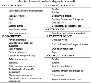
Leamer’s product classification system:
Scholar Leamer invented a product classification which is available to use in analysis of product space. He has divided products into 10 divisions as shown below.
Table 3-2. Leamer’s product category
1. ANIMAL PRODUCT 2. CEREAL
Live animals Cereal
Meat Feed
Dairy products Miscellaneous edible product
Fish Tobacco
Hides, skin Oil seed
Crude animal and vegetable
material Textile fibre
Animal and vegetable oils and fat Animal oils and fats
Animals, live (nes) Fixed vegetable oils and fat
3. CHEMICALS 4. LABOR INTENSIVE
Organic Non-metallic mineral
Inorganic Furnitur
Dyeing and tanning Travel goods, handbag
Medicinal and pharmaceutical Articles of apparel
Oils and perfume Footwear
Fertilizers Miscellaneous sophistication
Explosives Postal packet
Artificial resins and plastic Special transactions, not classified
Chemical materials, nes Coin
5. AGRICULTURE 6. FOREST PRODUCT
Vegetables and fruit Cork and wood
Sugar Pulp and waste paper
Coffee
Cork and wood, cork sophistications Beverage
Source: Jesus Philip (2010)
Latin America and Caribbean countries
[image:23.595.113.488.354.700.2]Table 3-2. Leamer’s product category (continued)
7. RAW MATERIAL 8. CAPITAL INTENSIVE
Crude fertilizer and crude minerals Leather Rubber
Metalliferous ore Textile yarn, fabrics
Coal Sanitary fixtures and fittings, nes
Gas Iron and steel
Electric curren Sophistications of metals, nes
Non-ferrous metal 9. PETROLEUM
Gold, non-monetar Petroleum and petroleum product
10. MACHINERY 11. FOREST PRODUCT
Power generating Cork and wood
Specialized for particular
industries Cork and wood, cork sophistications
Metalworking Pulp and waste paper
General industria Paper
Office and data processing 12. CAPITAL INTENSIVE
Telecommunication Leather
Electrical Rubber
Other transport equipments Textile yarn, fabrics
Professional and scientific
instruments Sanitary fixtures and fittings, nes
Photographic equipment Iron and steel
Armoured vehicles, firearms, and
ammunition Sophistications of metals, nes
Source: Jesus Philip (2010)
3.4
The Index of Opportunity
This index includes 4 dimensions such as sophistication, diversification, standardness and possibilities for exporting with comparative advantage over other products.
3.4.1 Export Sophistication
The first two factors that we consider in the Index of Opportunities are the sophistication level of the overall export basket (denoted EXPY) and the sophistication level of the core products (denoted EXPY-core). The EXPY core is included chemicals, machinery and metal products. It is easier different products taking advantage of ingredients in EXPY-core and gap between trees is near.
3.4.2 Diversification
Diversification indicates the number of products with RCA in export basket. Formally:
𝑛𝑢𝑚𝑏𝑒𝑟!.!,! = 𝑖!
!
!!!
𝑖!= 1 𝑖𝑓 𝑅𝐶𝐴! > 1
0 𝑜𝑡ℎ𝑒𝑟𝑤𝑖𝑠𝑒 (3-19)
where:
𝑛𝑢𝑚𝑏𝑒𝑟!.!,! - number of products with RCA of country 𝑐 in the year 𝑡;
𝑛 - number of products;
𝑖!
- product with RCA.
The diversification measures capability of product’s competitiveness in wide range. Also, for the EXPY-core, the diversification is measured by measurement which is similar to above. A question will come up that what about their diversifications of the EXPY-core are different when two countries have same diversifications. In this case, the country which has more diversifications in the EXPY-core has possibility to progress rapidly. Following ratio shall be applied in estimating it.
𝑟𝑎𝑡𝑖𝑜!,!=
𝑛𝑢𝑚𝑏𝑒𝑟!"#$
.!.!,! 𝑛𝑢𝑚𝑏𝑒𝑟!
.!,!
(3-20)
3.4.3 Standardness
Another special way of export basket is estimation on how many countries produces the particular product. It is named ‘standardness’ In other words, it determines whether the product is standard or not by that the product is produced by many country and fewer countries. Standardness of export basket of the country is shows as follows:
𝑠𝑡𝑎𝑛𝑑𝑎𝑟𝑑𝑛𝑒𝑠𝑠!,! = 1
𝑑𝑖𝑣𝑒𝑟𝑠𝑖𝑓𝑖𝑐𝑎𝑡𝑖𝑜𝑛!,!
𝑢𝑏𝑖𝑞𝑢𝑖𝑡𝑦!,!,!
!
(3-21)
where:
𝑠𝑡𝑎𝑛𝑑𝑎𝑟𝑑𝑛𝑒𝑠𝑠 - unique indicator of export basket of country 𝑐;
𝑑𝑖𝑣𝑒𝑟𝑠𝑖𝑓𝑖𝑐𝑎𝑡𝑖𝑜𝑛 - number of products with RCA is exported by the country; 𝑢𝑏𝑖𝑞𝑢𝑖𝑡𝑦 - number of countries which export product 𝑖 with RCA.
A lower value of standardness indicates that the country’s export basket is more unique.
3.4.4 Open Forest
the sophistication level of all potential exports of a country where the weight is the density or distance between each of these goods and those exported with comparative advantage.
3.5
Economic dependency and concentration index
Economic dependency index:
∆ 𝑀!"
∆𝐺𝐷𝑃! (3-22)
where:
𝑑 - country’s index;
𝑠 - group of other countries;
Δ - change operator;
𝑀 - import;
𝐺𝐷𝑃 - Gross Domestic Product.
In other words, numerator of the ratio is diversion of total import of country 𝑑 and
denominator is its diversion of GDP.
The Herfindahl-Hirschman Index (HHI):
𝐻= 𝑠!!
!
!!!
(3-23)
where:
𝑠! - market weight of firms;
𝑁 - group of other countries;
[image:26.595.109.486.606.677.2]The Herfindahl index ranges from 1/𝑁 to one and 𝑁 is number of firms competing in the market. Equivalently, if percents are used as whole numbers, as in 75instead of 0.75, the index can range up to 100!, or 10,000.
Table 3-3. Herfindahl-Hirschman Index
Herfindahl-Hirschman Index (HHI)< 0.01
(100) High competitive market
HHI < 0.15 (1,500) Unconcentrated market
0.15 (1500) <HHI <0.25 (2500) Moderate concentration
HHI > 0.25 (2500) High concentration
have unequal shares, the reciprocal of the index indicates the "equivalent" number of firms in
the industry. The normalized Herfindahl index ranges from 0 to 1.
4
Empirical Analysis
We intend to study the concentration of import and export by the Herfindahl-Hirschman Index, foreign trade flows by the Gravity model, comparative advantage by method RCA, Export package by the Opportunity Index and product space by the Tree and Monkey model, indentify contemporary situation of foreign trade and formulate a recommendation and research which are dedicated to increase economic benefits of foreign trade based on them in this section. In carrying out this analysis, data of International Trade Centre, Statistical Yearbook of National Statistical Office of Mongolia and Database COMTRADE of the United Nations are applied.
4.1
Economic Overview
4.1.1 Export and import structure
[image:27.595.124.472.426.577.2]The Russian Federation, People’s Republic of China, Japan, Republic of Korea, USA and Kazakhstan as importing countries are dominating and their portions in total import are stable. But, minerals and machinery are Mongolian main importation goods.
Figure 4-1. Import by countries
Source: National Statistical Office
Total amount of Mongolian import is growing up year to year except for decrease of 2009 in connection with world financial crisis.
0% 20% 40% 60% 80% 100%
1991 1995 1999 2003 2007 2011
Figure 4-2. Export by products
Source: National Statistical Office
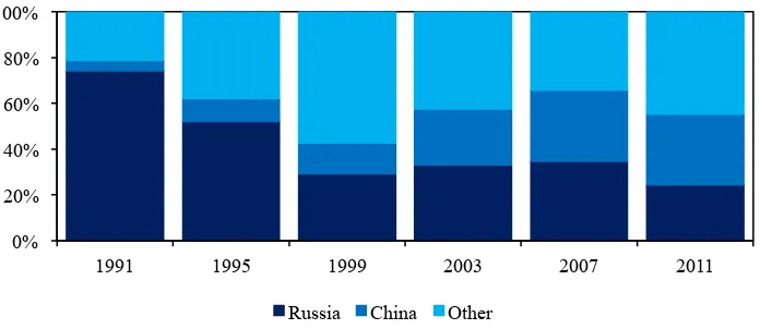
Over 80 percent of total export of Mongolia is occupied by People’s Republic of China and
about 80 percent of the export is minerals. It demonstrates that out country is increasingly depending on one country and one product for its exportation.
Figure 4-3. Export by countries, mil USD
Source: National Statistical Office
Like this, deepening of the concentration is causing the dependence of Mongolian economy on one country. It will constantly reduce efficiency and benefits of foreign trade.
4.1.2 Dependency and concentration analysis
Economic independency index: Growth of the independency index in recent years shows that our economy is increasingly depending on. Scholars have noticed that it is related to its import growth and the import is likely to expand in further.
0 1000 2000 3000 4000 5000 6000
0 1000 2000 3000 4000 5000 6000
2005 2006 2007 2008 2009 2010 2011
mi
ll
ion
U
S
D
mi
ll
ion
U
S
D
Other Metal Textiles Mineral Total export
0% 20% 40% 60% 80% 100%
1991 1995 1999 2003 2007 2011
[image:28.595.124.474.348.494.2]Figure 4-4. Economic independency
[image:29.595.118.470.279.442.2]Herfindahl-Hirshman index: There is not product concentration in its import. But, minor concentration in importing countries is observed. The concentration tends to increase in the future.
Figure 4-5. HHI, import by products
Figure 4-6. HHI, import by countries
[image:29.595.115.474.543.699.2]The concentration in export products is connected with export growth of industry in particular exploration sector. But, still increasing concentration in exporting countries is related to that large portion of export of exploration sector is being exported to China. Both of exporting countries and products have large amount of concentration and they are likely to constantly concentrate in further.
Figure 4-7. HHI, export by products
Figure 4-8. HHI, export by countries
0.4 0.5 0.6 0.7 0.8
1995 1996 1997 1998 1999 2000 2001 2002 2003 2004 2005 2006 2007 2008 2009 2010
0.00 0.05 0.10 0.15 0.20
1995 1998 2001 2004 2007 2010
0.00 0.05 0.10 0.15 0.20 0.25 0.30
1995 1998 2001 2004 2007 2010
0.00 0.10 0.20 0.30 0.40 0.50 0.60 0.70
1995 1998 2001 2004 2007 2010 0.00 0.20 0.40 0.60 0.80
4.1.3 Analysis of the Gravity model
[image:30.595.76.522.156.373.2]Following results are arisen by Panel data analysis on traditional and expanded Gravity model based on data of Mongolia between 2000 and 2010.
Table 4-1. Evaluation of expanded model
Variables Coefficients Standard mistakes Statistics Expectancy
C 259,3731 134,1416 1,933577 0,0553
GDPJ 0,202826 0,190419 1,065157 0,2887
GDPI 0,983932 0,765862 1,284738 0,2011
POPJ 0,079498 0,187756 0,423413 0,6727
POPI -19,05591 10,14604 -1,878163 0,0625
DIS -0,311207 0,282681 -1,100913 0,2729
EX (-1) 0,518975 0,080103 6,478882 0
EX (-2) 0,248457 0,084212 2,950371 0,0037
R^2 0,75197
AR^2 0,739013
DW 2,046876
CE FIXED
FE FIXED
The traditional model has more capability of explanation. According to the model, GDPs of two countries impacts on Mongolian export and gap between them is beneficial. These are consistent with theoretical hypothesis of the model.
Table 4-2. Evaluation of traditional model
Variables Coefficients Standard mistakes Statistics Expectancy
C 8,537881 5,685903 1,501587 0,1355
GDPJ 0,269031 0,121565 2,213068 0,0286
GDPI -0,403916 0,239938 -1,683419 0,0946
POPJ - - - -
POPI - - - -
DIS -0,3947 0,211209 -1,868769 0,0638
EX (-1) 0,528956 0,080397 6,579297 0
EX (-2) 0,24077 0,083937 2,868466 0,0048
R^2 0,745145
AR^2 0,735775
DW 2,107541
CE FIXED
FE FIXED
[image:30.595.77.522.461.678.2]4.1.4 Revealed comparative advantage analysis (as of 2010)
We analyze on RCA of productions and products based on data on Mongolian export and import between 2003 and 2010. RCA analysis of the comparative advantage of products that dedicated to production and consumers is the following (𝑅𝐶𝐴!,!" =𝑥, 𝑅𝐶𝐴!,!" =𝑚,
[image:31.595.76.525.190.309.2]𝑅𝐶𝐴!" = 𝑤).
Table 4-3. Mongolian industrial products for consumers and productions
2003 2004 2005 2006 2007 2008 2009 2010
Industrial products for consumers
x 0.846 0.738 0.614 0.421 0.323 0.315 0.333 0.200
m 1.173 1.209 1.126 1.401 1.360 1.254 1.578 1.310
w 0.721 0.610 0.545 0.300 0.237 0.251 0.211 0.153
Industrial products for production
x 3.920 3.467 3.416 4.073 4.105 2.837 2.872 2.002
m 1.652 2.036 1.774 1.620 1.457 1.283 1.157 1.543
w 2.372 1.702 1.925 2.514 2.816 2.211 2.482 1.297
[image:31.595.78.525.417.516.2]As above-mentioned, there is no comparative advantage in industrial goods that intended to consumers and production. However, it noticed that the certain goods of any groups have comparative advantages. Two out of the total 39 types of industrial goods for consumers have comparative advantages.
Table 4-4. Products with RCA within the products for consumers
2003 2004 2005 2006 2007 2008 2009 2010
Meat and offal
x 3.421 1.525 1.315 1.903 1.578 1.636 2.640 1.527
m 0.144 0.124 0.144 0.301 0.204 0.361 0.215 0.359
w 23.71 12.21 9.101 6.310 7.709 4.530 12.23 4.252
Animal products
x 21.03 18.80 17.08 10.38 8.819 8.268 9.461 5.816
m 0.111 0.197 0.158 0.389 0.039 0.239 0.011 0.212
w 188.1 95.18 107.7 26.63 223.2 34.52 822.4 27.31
In addition, 5 out of the total 48 types of industrial goods for production have comparative advantages.
Table 4-5. Products with RCA within the products for productions
2003 2004 2005 2006 2007 2008 2009 2010
Copper and copper products
x 0.716 1.184 1.067 0.973 1.071 1.472 1.204 1.108
m 0.072 0.061 0.066 0.033 0.061 0.068 0.089 0.063
w 9.926 19.24 15.93 29.28 17.42 21.41 13.40 17.44
Iron ore
x 72.49 70.98 53.37 63.78 65.89 62.91 52.41 29.91
m 0.043 0.010 0.005 0.002 0.002 0.138 0.001 0.004
w 1674 6870 9626 30171 23321 454.9 40767 6046
Metals
x 11.71 13.88 16.39 8.732 5.950 4.005 3.244 3.073
m 0.008 0.007 0.009 0.007 0.014 0.036 0.355 0.045
[image:31.595.80.522.593.762.2]