Conditional Market Timing in the Mutual Fund Industry

(1)

Munich Personal RePEc Archive

Conditional Market Timing in the

Mutual Fund Industry

Tchamyou, Vanessa and Asongu, Simplice

January 2017

Online at

https://mpra.ub.uni-muenchen.de/82633/

(2)

A G D I Working Paper

WP/17/028

Conditional Market Timing in the Mutual Fund Industry

Published in Research in International Business and Finance, 42, pp. 1355-136 (2017)

Vanessa S. Tchamyou

African Governance and Development Institute, P.O. Box 8413, Yaoundé, Cameroon. E-mail: simenvanessa@yahoo.com /

simenvanessa@afridev.org

Simplice A. Asongu

African Governance and Development Institute, P.O. Box 8413, Yaoundé, Cameroon. E-mail: asongusimplice@yahoo.com /

(3)

2017 African Governance and Development Institute WP/17/028

Research Department

Conditional Market Timing in the Mutual Fund Industry

Vanessa S. Tchamyou & Simplice A. Asongu

January 2017

Abstract

This study complements the scarce literature on conditional market timing in the mutual fund

industry by assessing determinants of market timing throughout the distribution of market

exposure. It builds on the intuition that the degree of responsiveness by fund managers to

investigated factors (aggregate liquidity, information asymmetry, volatility and market excess

return) is contingent on their levels of market exposure. To this end, we use a panel of 1467

active open-end mutual funds for the period 2004-2013. Fund-specific time-dynamic beta is

employed and we avail room for more policy implications by disaggregating the dataset into

market fundamentals of: equity, fixed income, allocation and tax preferred. The empirical

evidence is based on Quantile regressions. The following findings are established. First, there

is consistent positive threshold evidence of volatility and market return in market timing, with

the slim exception of allocation funds for which the pattern of volatility is either U- or

S-shaped. Second, the effect of volatility and market return are consistently positive and

negative respectively in the bottom and top quintiles of market exposure, but for allocation

funds. Third, the effects of information asymmetry and aggregate liquidity are positive and

negative, contingent on specifications, level of market exposure and market fundamentals.

The findings broadly suggest that blanket responses of market exposures to investigated

factors are unlikely to represent feasible strategies for fund managers unless they are

contingent on initial levels of market exposure and tailored differently across ‘highly

exposed’-fund managers and ‘lowly exposed’-fund managers. Implications for investors and fund managers are discussed.

(4)

1. Introduction

Over the past decades, the popularity of mutual funds has grown rapidly. Hence, instead of

getting into equity markets directly, investors have tended to prefer mutual funds (Wu, 2011).

Though, the performance of active mutual funds has been widely explored in the literature. In

other to deliver high performance, investment managers use different means like quantitative

methods, quantitative models plus additional information such as information on managers;

press articles or investment analysts (Bassett Jr & Chen, 2001). The assessment of the

performance is sometimes contingent on the market timing skills of managers of active

mutual funds.

Market timing is a situation where a timer seizes the opportunity of market fluctuations. He or

she can rebalance portfolio or switch asset allocations. Should the timer’s forecast market

expected return be accurate, he/she would be rewarded with a better performance relative to

benchmark portfolio characterised with a constant beta that is equivalent to the timer’s

portfolio average beta. Starting with the fundamental study of Trenor and Mazuy (1966),

several authors have worked on the ability of active mutual funds managers to time the

market. Trenor and Mazuy (1966) used a sample of 57 funds between 1957 and 1962 and

found evidence of timing ability only in one fund. They reached the conclusion that

investment managers cannot outguess the market. Considerable studies reached the same

conclusion of little evidence of market timing in the mutual fund industry. For instance, (1)

Kon (1983) found evidence of market timing at the individual fund level but no evidence

when funds are grouped; (2) Chang and Lewellen (1984) studied a sample of 67 monthly

mutual funds and found that only few fund managers seem to exhibit some ability to time the

market ; (3) Henriksson (1984) found evidence of market timing in only 3 funds out of the

118 studied and (4) Mansor et al. (2015) analysed 106 Malaysian equity funds and found that

evidence of market timing disappeared when employing panel regressions.

However, inquiries by Bollen and Busse (2001) have found evidence of market forecast

among managers of active mutual funds. Bollen and Busse (2001) emphasised the importance

of the frequency of data. Using daily data of 230 mutual funds, they found evidence of market

timing skill in a substantial numbers of funds. Applying holding-based measures, Jiang et al.

(2007) found a positive timing ability of mutual fund managers. It is important to note that

their sample is only made of equity funds.

Every fund managers do not time the market exactly the same way since they do not have

(5)

information each fund manager has. Some studies in the existing literature have employed

conditional market timing to assess the performance of funds in terms of market timing skill.

The concept of conditional market timing has been explored in different perspectives, but

mostly conditioned on public versus private information. Ferson and Schadt (1996) advocate

the conditional performance evaluation of mutual funds, conditioned on public information.

They use a sample of 67 monthly mutual funds for the period 1968-1990 and their findings

reveal statistical and economical results when applying conditional information. Therefore,

the responsiveness of funds to public information changes with risk exposure. More recently,

Dahr and Mandal (2014) have also employed the conditional performance evaluation to

investigate the performance of Indian mutual funds with respect to the ability of fund

managers to forecast the market. Using 80 mutual funds schemes over the period 2000-2012,

they found that the conditioning on public information improves the coefficient of

determination when applying the unconditional Henriksson-Merton and Treynor-Mazuy

models under the same period.

The findings of Dahr and Mandal run counter to those earlier established by Becker et al.

(1999) on the evidence of market timing skills from active mutual fund managers. They made

a distinction between timing based on publicly available information which can be captured

by some instrumental variables and timing based on better information. They call the latter

“Conditional market timing”. Analysing a sample of 400 U.S. mutual funds over 1976 – 1994 period, with conditioning based on public information, they find that mutual funds are highly

risk averse and no evidence of a significant timing ability in the market. Taking into account

the conditional perspective, Saez (2008) and Holmes and Faff (2004) also found very little

evidence of market timing ability.

The engaged literature clearly leaves room for improvement on two fronts, namely: the need

to assess market timing in the mutual fund industry beyond equity funds on the one hand and

on the other hand, assess how market factors affect market timing when existing levels of

market timing are considered. To put the above points into more perspective, as discussed

above, the concept of market timing has been more studied with equity funds for the most

part. However, the timing ability of funds managers should not be limited only to equity funds

(Elton et al., 2011). Hence, we complement equity funds with fixed income, allocation, tax

preferred funds.

This study contributes to the literature by investigating the roles of information asymmetry

and other factors on market timing throughout the conditional distribution of market timing.

(6)

managers with low market exposure to the conditioning information set (aggregate liquidity;

information asymmetry and volatility) should intuitively be different from managers that are

characterised with higher market exposure. Moreover, it is very likely that fund managers

with low market exposure are associated with a higher level of information asymmetry and

vice versa. Hence, from logic and intuition, the response of fund managers to information

asymmetry is very likely to be contingent on the level of market exposure fund managers are

acquainted with.

The rest article is organised as follows. Data, methodology and estimation procedure

are presented in section 2. Section 3 documents the empirical analysis and results. Section 4

presents concluding implications and future research directions.

2. Data and methodology 2.1 Data

We analyse annual open-end mutual fund returns from the Morningstar Direct database for

the period 2004 to 2013. We divide our sample into four sub-samples based on the Global

Broad Category Group of Morningstar: equity, fixed-income, allocation and tax-preferred

funds. We study each sub-sample in detail to compare the responsiveness of fund managers to

each type of fund on the conditional distribution of market exposure.

We apply a filter to remove all missing values due to methodological constraint and end-up

with a strongly balanced panel dataset of 882 equity funds, 243 fixed-income funds, 156

allocation funds and 186 tax-preferred funds. As result, we have 1467 active mutual funds for

(7)

[image:7.595.84.511.148.366.2]

Table 1 Summary statistics

This table presents the Summary statistics of variables used in our analysis in panel A and fund categories in panel B. Std. Dev.: Standard Deviation. Min.: Minimum. Max. : Maximum. Obs.: Observations.

Panel A : Variables

Obs. Mean Std. Dev. Min. Max.

Beta 8928 -0.018 0.932 -4.502 4.571

Info. Asymmetry 8928 19.467 15.245 0.000 93.425

Volatility 7440 19.467 12.115 0.691 64.902

Mkt Excess Return 14880 8.578 19.038 -38.39 35.15

Aggregate Liquidity 14880 -0.025 0.028 -0.098 0.010

SMB 14880 3.003 7.485 -7.01 17.74

HML 14880 2.411 12.342 -21.55 23.66

Panel B: Fund categories

Equity 14880 0.592 0.491 0 1

Fixed income 14880 0.163 0.369 0 1

Allocation 14880 0.104 0.306 0 1

Tax preferred 14880 0.125 0.330 0 1

SMB: Size. HML: Book to market. Std. Dev.: Standard Deviation. Min.: Minimum. Max. : Maximum. Obs.: Observations.

The summary statistics for various types of mutual fund and variables are discussed in

Panel A and Panel B respectively of Table 1. Two motivations underpin the summary

statistics. One on the hand, it is apparent that the variables are comparable from the

perspective of mean values. On the other hand, corresponding variations from the standard

deviations is an indication that we can be confident that reasonable estimated linkages will

result from the empirical analysis.

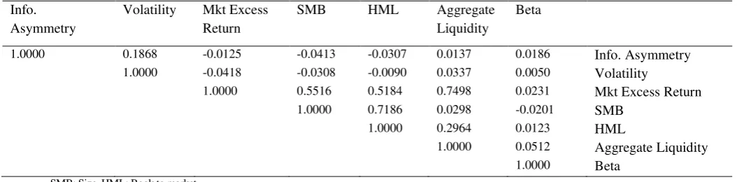
Table 2 discloses the correlation matrix. It enables the study to avoid concerns about

multicollinearity that could lead to variables with a high degree of substitution entering into

conflict and reflecting unexpected signs in the estimation output. Therefore, in specifications

of the main equation, ‘aggregate liquidity’ and ‘market excess return’ are not involved the

same estimation owing their high degree of substitution. This is consistent with a caution from

Cao et al. (2013, p. 285) that high market return is strongly associated with market liquidity.

In accordance with Bodson et al. (2013), book-to-market and market size are entered into the

same equation when estimating the beta variable for market timing.

[image:7.595.85.515.148.366.2]

(8)

[image:8.595.35.562.122.252.2]

Table 2 Correlation matrix

This table presents the correlation matrix of variables used in our analysis Info.

Asymmetry

Volatility Mkt Excess Return

SMB HML Aggregate

Liquidity

Beta

1.0000 0.1868 -0.0125 -0.0413 -0.0307 0.0137 0.0186 Info. Asymmetry

1.0000 -0.0418 -0.0308 -0.0090 0.0337 0.0050 Volatility

1.0000 0.5516 0.5184 0.7498 0.0231 _{Mkt Excess Return}

1.0000 0.7186 0.0298 -0.0201 _SMB

1.0000 0.2964 0.0123 _HML

1.0000 0.0512 Aggregate Liquidity

1.0000 Beta

SMB: Size. HML: Book to market.

2.2 Methodology

2.2.1 Estimation of volatility, beta and information asymmetry

Various measurements for information asymmetry have been proposed in the literature.

Tchamyou and Asongu (2017), Asongu et al. (2016) have used private credit bureaus and public

credit registries as proxies for ‘reducing information asymmetry’ in the banking industry. Dai et

al. (2013) have employed the standard deviation of return’s idiosyncratic risk to investigate how

mutual fund ownership and information asymmetry affect the management of earnings by listed

companies. In accordance with the same definition, the cost originating from information

asymmetry between elements of a syndicated bank loan has been examined by Ivashina (2009).

Dierken (1991) has used four indicators to appreciate information asymmetry between the market

and firm managers within the context of equity. What is common among these studies is the fact

that information asymmetry is proxied as the difference between realised and expected returns.

This study is in line with the underlying intuition for the estimation of uncertainty in information

as well as asymmetric information. Therefore, we compute information asymmetry as the

standard deviation of the idiosyncratic risk of returns1. Within this context, asymmetric

information corresponds to the standard deviations of individual returns’ residuals, in which case

standard errors are equal to the standard deviation of residuals. Accordingly, whereas the Capital

Asset Pricing Model (CAPM) augmented with the Fama-French 3-factor model (here after FF)

(see Eq.2 below) is employed for the computation of asymmetric information, a stochastic

modelling estimation process is used to derive volatility or uncertainty. The approach we adopt

1

(9)

for the of estimation volatility, beta and information asymmetry is consistent with Tchamyou et al.

(2017).

Returns’ volatility is estimated as the standard errors corresponding to the first order auto-regressive processes of the returns. In accordance with Kangoye (2013), owing to the low

frequency nature of our data, volatilities or uncertainties cannot be computed with GARCH

(Generalized Auto-Regressive Conditional Heteroskedasticity) models. Hence, auto-regressive

estimations are employed. It follows that the Kangoye (2013) estimation process is employed to

estimate volatility because the dataset consists of open-end mutual funds of annual periodicity.

Therefore, uncertainty corresponds to the saved RMSE2 (Root-Mean_Square Error) of each return

obtained from the first autoregressive processes. The computation process is summarised in the

following equation. t i t i t

i R T

R_, 







_,_₁ 







_, , (1)

where Ri,t is the return of fund i at time

t

; Ri,t1 the return of fund i at time t1 ; Tthe time

trend; the constant ;



the parameter and



i,t the error term.

We model mutual fund returns with the FF three factors model to estimate fund-specific

systematic risk. t i t i HML t i SMB t t i MKT i t f t

i R MKT SMB HML

R_,  _, 







_,_, 



_, 



_, 



_, , (2)

where Rf is the risk free rate. MKTis the market excess return, SMB Small [market

capitalization] Minus Big and HML High [book-to-market ratio] Minus Low. The previous 3

factors are taken from the Kenneth French's website3.

A simple view of information asymmetry can then be modelled as follows:

      _  _i_t _i_t

t

i R R

IA_,



_, _,

(3)

Where IAis Information Asymmetry;  the standard deviation; Ri,t the realised return of

fund i at time

t

;



t i

R_, the expected return computed using the FF 3 factor model.

The dynamic beta corresponding to each mutual fund is estimated as a proxy for market exposure

or market time. The advantage of employing betas is that it captures more market heterogeneities

because in each year a distinct beta is computed for each fund. It is important to note that

2

The RMSE (Root-Mean-Square Error) can be employed as a measure of uncertainty or as the standard deviation of residuals (see Kitagawa & Okuda, 2013).

3

(10)

static beta have the shortcoming of failing to capture some inherent variations that could

substantially help in the elucidation of the market timing ability of fund managers. In essence, the

mainstream literature has cautioned that assets’ betas may vary over time (see Ferson & Schadt,

1996, p. 428). Using the Rollreg Stata command, we estimate the time-varying beta and RMSE

for asymmetric information in Equation 2. Considering that there is a time-window that is higher

than the number of independent indictors by at least one degree of freedom, a five-year

moving-window is adopted because four missing observations are apparent in each fund. It is important to

note that four observations are automatically missing because we are using four independent

variables of interest.

In order to estimate the indicator of liquidity, the aggregate liquidity factors from an updated

series by Pástor and Stambaugh (2003) are used. Consistent with Bodson et al. (2013), all factors

are retrieved from the website of Robert Stambaugh4. Given that liquidity data is in months,

whereas the mutual fund data is annual, annual averages are computed with the monthly data.

2.2.2. Estimation technique

Consistent with the motivation of the study, estimation techniques that are based on mean

values of market timing can only result in blanket practical implications for fund managers.

Hence, approaches based on mean values of the dependent variable like Ordinary Least

Squares (OLS) and the Generalised Method of Moments (see Tchamyou et al., 2017) reflect

the underlying shortcoming. Accordingly, they estimate the linear conditional mean functions

and articulate the central trend of the dependent variables. Consequently, they do not take into

account the distribution of the tails. Hence, a Quantile Regression (QR) approach is applied in

this study to address the discussed shortcomings from estimation techniques that are based on

mean values of the market timing’s distribution. In essence, the QR is employed in this study

to investigate the determinants of market exposure throughout the conditional distribution of

market timing (Keonker & Hallock, 2001). The QR is based on median regression and was

developed by Koenker and Bassett (1978). While the OLS supposes the normal distribution

between the error term and the dependent variables, the QR is not established on this

hypothesis. According to Lee and Saltoglu (2001), the main advantage of the QR technique is

its capacity of producing more robust estimates (Koenker & Basett, 1982). The application of

QR is increasing in the finance literature, notably in: (i) analysing risk in mutual funds (Wang

4

(11)

et al., 2015) and (ii) examining the relationship between fund governance and performance

(Chen & Huang, 2011).

In accordance with recent QR literature (Efobi & Asongu, 2016; Asongu et al., 2017),

the th quintile estimator of market timing is obtained by solving for the following optimization problem, which is presented without subscripts in Eq. (3) for ease of

presentation.    





















          









 i i i i i i k x y i i i x y i i i R

x

y

x

y

: :

)

1 (

min

, (4)

where

 

0,1 . Contrary to OLS that is fundamentally based on minimizing the sum

of squared residuals, with QR, we minimize the weighted sum of absolute deviations. For

instance the 10th or 90th quintiles (with =0.10 or 0.90 respectively) by approximately weighing the residuals. The conditional quintile of market timing oryigiven xiis:





 i i

y x x

Q ( / )  , (5)

where unique slope parameters are modelled for each th specific quintiles. This formulation is analogous to E(y/x) xi in the OLS slope where parameters are examined only at the

mean of the conditional distribution of market timing. For the model in Eq. (5), the dependent

variable yi is the market timing indicator, while xi contains a constant term, information

asymmetry, market excess return and aggregate liquidity.

3. Empirical results

While Table 3 presents findings corresponding to the full sample, the results of the remaining

tables pertain to sub-samples. Accordingly, Table 4, Table 5, Table 6 and Table 7

respectively correspond to equity funds, fixed income funds, tax-preferred funds and

allocation funds. There are two main specifications corresponding to each table: one

specification without aggregate liquidity and another specification without market excess

return. The two specifications are used to address the apparent concern of multicollinearity or

high degree of substitution between market excess return and aggregate liquidity.

For all tables disclosing the empirical results, consistent difference in estimates from market

exposure determinants between OLS and quintiles (in terms of sign, significance and

magnitude of significance) justify the relevance of adopted empirical strategy. Since, the

(12)

market exposure, the corresponding trend in tendencies could take several patterns, inter alia:

S-shaped, U-shaped, inverted U-shaped and positive or negative threshold shapes. The notion

of threshold adopted in this study is consistent with Asongu (2014). In essence, a positive

threshold is apparent when throughout the distribution of market exposure, the estimates

consistently display decreasing negative magnitudes and/or increasing positive magnitudes. In

the same vein, a negative threshold is established when an estimated coefficient consistently

displays decreasing positive and/or increasing negative magnitudes throughout the conditional

distribution of market exposure. In other words, a positive threshold denotes consistent

incremental effects of the underlying estimate on market exposure.

The following findings can be established from Table 3 which shows results of the full

sample. First, information asymmetry significantly affects market exposure in the bottom

quintiles, with a negative (positive) effect (s) in the 10th (25th and 50th) quintile(s). Second,

positive thresholds are apparent from the effects of volatility and market excess return. Third,

aggregate liquidity has a positive effect on market exposure in the top quintiles.

In Table 4 which shows results of the equity funds sub-sample, the findings of the full sample

are broadly confirmed with the exception that the positive effect from aggregate liquidity is

now also significant in the 25th and 50th quintiles. Looking at Table 5 which shows results of

the fixed-income funds sub-sample, the findings of the full sample are broadly confirmed with

the exception that the effect of information asymmetry is consistently negative in the top

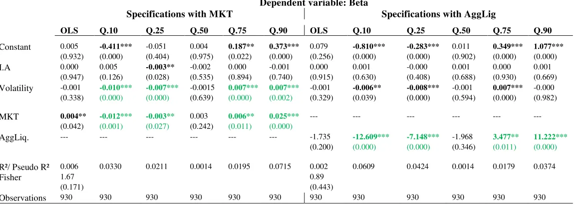
quintiles of the market exposure distribution. From Table 6 on the results of the tax-preferred

funds sub-sample, findings of the full sample are broadly confirmed with the exception that

the effect of aggregate liquidity is not negative (positive) in the top quintiles of market

exposure. In Table 7 which presents findings of the sub-sample corresponding to allocation

funds: (i) information asymmetry positively affects market exposure from the 10th to the 50th

quintiles; (ii) the incidence of volatility is U-shaped on the left-hand-side and S-shaped in the

right-hand-side; (iii) market excess return displays a positive threshold effect from the 25th to

the 90th quintiles whereas aggregate liquidity positively (negatively) affects market exposure

(13)

[image:13.595.39.588.166.364.2]

Table 3

Quantile regression based on full sample

This table presents the quantile regression of the determinants of market timing.

*, **, ***: significance levels of 10%, 5% and 1% respectively. P-values are in brackets. OLS: Ordinary Least Squares. R² is for OLS and Pseudo R² for Quantile regression. I.A: Information Asymmetry. MKT: Market Excess Return. AggLiq: Aggregate Liquidity. Lower quantiles (e.g., Q 0.10) signify fund where market exposure is least.

Dependent variable: Beta

Specifications with MKT Specifications with AggLig

OLS Q.10 Q.25 Q.50 Q.75 Q.90 OLS Q.10 Q.25 Q.50 Q.75 Q.90

Constant -0.000 -0.030 -0.105** 0.050 0.059** 0.133*** 0.001 -0.552*** -0.317*** 0.010 0.302*** 0.674***

(0.999) (0.386) (0.020) (0.208) (0.032) (0.004) (0.964) (0.000) (0.000) (0.733) (0.000) (0.000)

I.A 0.001** -0.003*** 0.001 0.002*** 0.000 -0.000 0.001** 0.001 0.002** 0.002*** -0.000 -0.001 (0.041) (0.000) (0.215) (0.003) (0.149) (0.683) (0.027) (0.115) (0.046) (0.001) (0.769) (0.233)

Volatility -0.000 -0.026*** -0.013*** -0.001 0.015*** 0.023*** -0.000 -0.023*** -0.013*** -0.001 0.014*** 0.022***

(0.968) (0.000) (0.000) (0.146) (0.000) (0.000) (0.905) (0.000) (0.000) (0.129) (0.000) (0.000)

MKT -0.001 -0.020*** -0.010*** -0.002*** 0.006*** 0.021*** --- --- --- --- --- ---

(0.105) (0.000) (0.000) (0.008) (0.000) (0.000)

AggLiq. --- --- --- --- --- --- 2.630*** -0.881 -1.395 0.761 6.090*** 10.219***

(0.000) (0.194) (0.108) (0.267) (0.000) (0.000)

R²/ Pseudo R² 0.001 0.089 0.024 0.001 0.029 0.078 0.002 0.0403 0.0144 0.001 0.032 0.043

Fisher 2.56* 9.00***

(0.053) (0.000)

Observations 7440 7440 7440 7440 7440 7440 7440 7440 7440 7440 7440 7440

Table 4

Quantile regression based on equity funds

This table presents the quantile regression of the determinants of market timing based on equity funds.

Constant 0.157*** -0.078 0.024 0.283*** 0.188*** 0.272*** 0.072* -0.683*** -0.275*** 0.131*** 0.356*** 0.711***

(0.001) (0.135) (0.621) (0.000) (0.000) (0.000) (0.057) (0.000) (0.000) (0.007) (0.000) (0.000)

I.A 0.001* -0.004*** 0.001 0.002** 0.000 -0.000 0.002** 0.002 0.002* 0.002* -0.000 0.000 (0.096) (0.000) (0.139) (0.019) (0.669) (0.717) (0.022) (0.313) (0.054) (0.052) (0.426) (0.617)

Volatility -0.003** -0.023*** -0.019*** -0.003** 0.016*** 0.020*** -0.003** -0.024*** -0.018*** -0.004*** 0.015*** 0.020***

(0.020) (0.000) (0.000) (0.010) (0.000) (0.000) (0.012) (0.000) (0.000) (0.002) (0.000) (0.000) MKT -0.007*** -0.024*** -0.016*** -0.011*** 0.002* 0.022*** --- --- --- --- --- ---

(0.000) (0.000) (0.000) (0.000) (0.060) (0.000)

AggLiq. --- --- --- --- --- --- 4.562*** -0.883 3.076*** 0.131*** 6.573*** 7.035***

(0.000) (0.589) (0.001) (0.007) (0.000) (0.000)

R²/ Pseudo R² 0.008 0.111 0.042 0.011 0.018 0.067 0.007 0.036 0.023 0.003 0.025 0.031

Fisher 9.67*** 14.20***

(0.000) (0.000)

[image:13.595.7.596.518.714.2]

(14)

[image:14.595.46.588.166.349.2]

Table 5

Quantile regression based on fixed-income funds

This table presents the quantile regression of the determinants of market timing based on fixed-income funds.

*, **, ***: significance levels of 10%, 5% and 1% respectively. P-values are in brackets. OLS: Ordinary Least Squares. R² is for OLS and Pseudo R² for Quantile regression. IA: Information Asymmetry. MKT: Market Excess Return. AggLiq: Aggregate Liquidity. Lower quantiles (e.g., Q 0.10) signify fund where market exposure is least.

Constant -0.206*** -0.067 -0.035 -0.012 -0.080 -0.111 0.042 -0.256*** -0.048 0.113*** 0.321*** 0.878***

(0.007) (0.401) (0.544) (0.819) (0.197) (0.356) (0.406) (0.000) (0.285) (0.001) (0.000) (0.000) I.A -0.003* 0.004 0.002 -0.001 -0.004** -0.008*** -0.004* 0.005 0.003* -0.000 -0.007*** -0.009***

(0.087) (0.126) (0.116) (0.271) (0.012) (0.004) (0.056) (0.101) (0.085) (0.572) (0.000) (0.000) Volatility 0.002 -0.029*** -0.025*** -0.009*** 0.014*** 0.032*** 0.002 -0.029*** -0.024*** -0.010*** 0.013*** 0.022***

(0.385) (0.000) (0.000) (0.000) (0.000) (0.000) (0.459) (0.000) (0.000) (0.000) (0.000) (0.000)

MKT 0.009*** -0.011*** 0.000 0.008*** 0.013*** 0.025*** --- --- --- --- --- --- (0.000) (0.000) (0.829) (0.000) (0.000) (0.000)

AggLiq. --- --- --- --- --- --- 4.077*** 2.396 -0.706 -0.781 5.885*** 17.681***

(0.001) (0.184) (0.557) (0.351) (0.000) (0.000)

R²/ Pseudo R² 0.016 0.108 0.055 0.023 0.061 0.166 0.008 0.088 0.055 0.015 0.048 0.113

Fisher 5.16*** 3.98***

(0.001) (0.007)

Observations 1215 1215 1215 1215 1215 1215 1215 1215 1215 1215 1215 1215

Table 6

Quantile regression based on tax-preferred funds

This table presents the quantile regression of the determinants of market timing based on tax-preferred funds.

Constant 0.005 -0.411*** -0.051 0.004 0.187** 0.373*** 0.079 -0.810*** -0.283*** 0.011 0.349*** 1.077***

(0.932) (0.000) (0.404) (0.975) (0.022) (0.000) (0.256) (0.000) (0.000) (0.902) (0.000) (0.000)

I.A 0.000 0.005 -0.003** -0.002 0.000 -0.001 0.000 0.001 -0.000 0.001 0.000 0.001

(0.947) (0.126) (0.028) (0.535) (0.894) (0.740) (0.915) (0.630) (0.408) (0.688) (0.930) (0.669)

Volatility -0.001 -0.010*** -0.007*** -0.0015 0.007*** 0.007*** -0.001 -0.006** -0.008*** -0.001 0.007*** -0.000

(0.338) (0.000) (0.000) (0.639) (0.000) (0.002) (0.329) (0.039) (0.000) (0.594) (0.000) (0.982)

MKT 0.004** -0.012*** -0.003** 0.003 0.006** 0.025*** --- --- --- --- --- --- (0.042) (0.001) (0.027) (0.242) (0.011) (0.000)

AggLiq. --- --- --- --- --- --- -1.735 -12.609*** -7.148*** -1.968 3.477** 11.222***

(0.200) (0.000) (0.000) (0.346) (0.011) (0.000)

R²/ Pseudo R² 0.006 0.0330 0.0211 0.0014 0.0195 0.0715 0.002 0.0609 0.0424 0.0014 0.0179 0.0374

Fisher 1.67 0.89

(0.171) (0.443)

[image:14.595.14.596.510.716.2]

(15)

[image:15.595.17.586.191.387.2]

Table 7

Quantile regression based on allocation funds

This table presents the quantile regression of the determinants of market timing based on allocation funds.

Constant -0.534*** -1.263*** -0.645*** -0.324*** -0.157 0.018 -0.512*** -1.311*** -1.118*** -0.381*** -0.077 0.310***

(0.000) (0.000) (0.000) (0.000) (0.152) (0.868) (0.000) (0.000) (0.000) (0.000) (0.229) (0.000)

I.A 0.006*** 0.012*** 0.011*** 0.006*** 0.000 -0.000 0.006*** 0.014*** 0.010*** 0.007*** 0.000 -0.001 (0.000) (0.000) (0.000) (0.000) (0.648) (0.849) (0.000) (0.000) (0.000) (0.000) (0.708) (0.728)

Volatility 0.017*** 0.013*** 0.011*** 0.009*** 0.021*** 0.033*** 0.017*** 0.010*** 0.018*** 0.010*** 0.024*** 0.034***

(0.000) (0.000) (0.000) (0.000) (0.000) (0.000) (0.000) (0.004) (0.000) (0.000) (0.000) (0.000)

MKT 0.003 -0.001 -0.010*** 0.004*** 0.008*** 0.013*** --- --- --- --- --- ---

(0.169) (0.558) (0.000) (0.003) (0.003) (0.000)

AggLiq. --- --- --- --- --- --- -3.795** -5.651** -7.974*** -2.117 -2.611* 6.583**

(0.013) (0.016) (0.000) (0.186) (0.054) (0.012)

R²/ Pseudo R² 0.092 0.045 0.076 0.059 0.080 0.117 0.096 0.052 0.085 0.057 0.072 0.094

Fisher 32.04*** 27.78***

(0.000) (0.000)

Observations 780 780 780 780 780 780 780 780 780 780 780 780

4. Concluding implications and future research direction

This study has complemented the scarce literature on conditional market timing in the mutual

fund industry by assessing determinants of market timing throughout the conditional

distribution of market exposure. It builds on the intuition that the degree of responsiveness by

fund managers to investigated factors (aggregate liquidity, information asymmetry, volatility

and market excess return) is contingent on their levels of market exposure. To this end, we

have used a panel of 1467 active open-end mutual funds for the period 2004-2013.

Fund-specific time-dynamic beta has been employed and we have availed room for more policy

implications by disaggregating the dataset into market fundamentals of: equity, fixed income,

allocation, tax preferred. The empirical evidence is based on Quantile Regressions.

The following findings have been established. First, there is a consistent positive threshold

evidence of volatility and market return in market timing, with the slim exception of

allocation funds for which the pattern of volatility is either U- or S-shaped. Second, the effect

of volatility and market return are consistently positive and negative respectively in the

bottom and top quintiles of market exposure, with the exception of allocation funds. Third, the

effects of information asymmetry and aggregate liquidity are positive and negative,

(16)

The notion of threshold adopted in the study is such that, a positive threshold is apparent

when throughout the distribution of market exposure, the estimates consistently display

decreasing negative magnitudes and/or increasing positive magnitudes. In the same vein, a

negative threshold is established when an estimated coefficient consistently displays

decreasing positive and/or increasing negative magnitudes throughout the conditional

distribution of market exposure. In other words, positive thresholds denote consistent

incremental effects of the underlying estimate on market exposure.

Our findings, especially threshold evidence have confirmed the fact that the effect of

information asymmetry and other determinants of market exposure are contingent on existing

levels of market exposure. Hence, ceteris paribus, with the same information on volatility and

market excess return, a fund manager who is already comparatively more exposed to the

market is very likely to increase his/her market exposure at a higher rate compared to his/her

counterpart who is less exposed to the market. Hence, the degree of sensitivity to market

exposure from market excess return and market volatility is a positive function to exiting

levels in market exposure.

In the light of the above, the degree of responsiveness by fund managers with low market

exposure to the investigated factors (aggregate liquidity; information asymmetry and

volatility) should intuitively be different from those from their counterparts with higher

market exposure. This information is critical in the understanding of fund managers’

behaviour towards or reaction to common market information. Hence, policy makers who

have been viewing fund managers’ market exposure reactions to market information

regardless of their initial levels of market exposure may be getting their dynamics badly

wrong.

The findings related to market volatility and market excess return have implications for

arbitrage and portfolio diversification in the perspective that, with information on market

excess return and market volatility if an investor judges that the returns to more market

exposure outweigh potential risks, everything being equal; engaging with fund managers that

are more exposed to the market is more likely to reward the underlying investors. Conversely,

if the investor judges that the risk/return advantage associated with more market exposure is

great, with the same information on market excess return and market volatility, the investor is

more likely to engage with fund managers that have less exposure to the market compared to

their counterparts that are more exposed. The underlying patterns from our findings could

enable a market timer to switch asset allocations and/or rebalance portfolios depending on

(17)

The above policy implications should also be contingent on the following trends: (i) the effect

of information asymmetry is driven by the equity funds sub-sample; (ii) the impact of market

volatility and market excess return are driven by equity and fixed-income sub-samples for the

most part while (iii) the effect of aggregate liquidity is driven by the fixed income funds

sub-sample. Moreover, the fact that the incidences of market return and volatility are consistently

negative and positive respectively in the top and bottom quintiles of market exposure further

substantiate the suggested practical recommendations in arbitrage and portfolio

diversification. Overall, the findings broadly suggest that blanket responses of market

exposure to investigated factors are unlikely to represent feasible strategies for fund managers

unless they are contingent on initial levels of market exposure and tailored differently across

‘highly exposed’-fund managers and ‘lowly exposed’-fund managers.

Future studies can focus on assessing thresholds at which various determinants of market

timing influence fund managers’ market timing ability both at the conditional mean and conditional distribution of market exposure. This future direction will provide insights into

whether the signs of the determinant change when certain levels of the underlying

(18)

Appendices

Appendix 1 Definition of Variables

Variables Signs Definitions Sources

Market timing Beta Measure of systematic risk. Computed

Information Asymmetry

Info. Asymmetry (IA)

Standard deviation of the idiosyncratic risk of individual return.

Computed

Volatility Vol. Measure of dispersion of return (or uncertainty) of a security.

Computed

Market Excess Return

Mkt Excess Return Difference between the return of the market and the risk free rate.

Kenneth French's website

Size SMB Small [market capitalization] Minus Big.

Book-to-market HML High [book-to-market ratio] Minus Low.

Aggregate Liquidity Agg.Liq. “Our monthly aggregate liquidity measure is a cross-sectional average of individual- stock liquidity measures” (Pástor and Stambaugh, 2003, p.643).

Robert Stambaugh's Website

Mutual fund categories

Variables Definitions Source

Equity “Global equity portfolios invest in companies domiciled in developed countries throughout the world. Some of these portfolios may include emerging market countries”.(p.9)

Morningstar Fixed-income “Global fixed income portfolios invest in fixed income securities from countries

domiciled in developed countries throughout the world. Some of these portfolios may include fixed income securities of emerging market countries”.(p.20)

Allocation “Allocation portfolios seek to provide both capital appreciation and income by investing in three major areas: stocks, bonds, and cash. While these portfolios explore the whole world, most of them focus on the U.S., Canada, Japan, and the larger markets in Europe. These portfolios typically have at least 10% of assets in bonds and less than 70% of assets in stocks.”(p.15)

(19)

References

Asongu, S. A., (2014). “Financial development dynamic thresholds of financial

globalisation: evidence from Africa”, Journal of Economic Studies, 41(2), pp. 166-195.

Asongu, S. A., Nwachukwu, J., & Tchamyou, V. S., (2016). “Information Asymmetry and

Financial Development Dynamics in Africa”. Review of Development Finance. 6(2), pp. 126-138.

Asongu, S. A., Anyanwu, J. C., & Tchamyou, V. S., (2017). “Technology-driven information sharing and conditional financial development in Africa”, Information Technology for Development. DOI: 10.1080/02681102.2017.1311833.

Bassett Jr., G.W., & Chen, H-L., (2001). “Portfolio Style: Return-Based Attribution Using Quantile Regression”. Economic Applications of Quantile Regression, pp.293-305.

Becker, C., Ferson, W.E., Myers, D.H. & Schill, M.J., (1999). “Conditional market timing with benchmark investors”. Journal of Empirical Finance, 52(1), pp.119-148.

Bodson, L., Cavenaile, L. & Sougné, D., (2013). “A global approach to mutual funds market

timing ability”. Journal of Empirical Finance, 20(January), pp.96–101.

Bollen, N.P.B. & Busse, J.A., (2001). “On the Timing Ability of Mutual Fund Managers”. Journal of Finance, 56(3), pp.1075-1094.

Chang, E., & Lewellen, W., (1984). “Impact of size and flows on performance for funds of hedge funds”. Journal of Business, 57(1), pp.57-72.

Chen, C. R., & Huang, Y., (2011). “Mutual Fund Governance and Performance: A Quantile Regression Analysis of Morningstar's Stewardship Grade”. Corporate Governance: An International Review, 19(4), pp.311-333.

Dai, Y., Kong, D. & Wang, L., (2013). “Information asymmetry, mutual funds and earnings management: Evidence from China”. China Journal of Accounting Research, 6(3), pp.187-209.

Dhar, J., & Mandal, K., (2014). “Market timing abilities of Indian mutual fund managers: an empirical analysis”. Indian Institute of Management, 41(3), pp.299-311.

Dierkens, N., (1991). “Information Asymmetry and Equity Issues”. Journal of Financial and Quantitative Analysis, 26(2), pp.181–199.

Efobi, U., & Asongu, S. A., (2016). “Terrorism and capital flight from Africa”, International Economics, 148 (December), pp. 81-94 (December, 2016).

(20)

Ferson, W.E., & Schadt, R.W., (1996). “Measuring fund strategy and performance in changing economic conditions”. Journal of Finance, 51(2), pp.425–461.

Henriksson, R.D., (1984). “Market Timing and Mutual funds perfomance: An Empirical Investigation”. Journal of Business, 57(1, Part 1), pp.73–96.

Holmes, K.A., & Faff, R.W., (2004). “Stability, asymmetry and seasonality of fund performance: an analysis of Australian multi-sector managed funds”. Journal of Business Finance and Accounting, 31(3&4), pp.539–578.

Ivashina, V., (2009). “Asymmetric information effects on loan spreads”. Journal of Financial Economics, 92(2), pp.300–319.

Jiang, G., Yao, T., & Yu, T., (2007). “Do mutual funds time the market? Evidence from portfolio holdings”. Journal Financial Economics, 86 (3), pp.724–758.

Kitagawa, N. & Okuda, S., (2016). “Management Forecasts, Idiosyncratic Risk, and Information Environment”, The International Journal of Accounting, 51(4), pp. 487–503.

Kangoye, T., (2013). “Does aid unpredictability weaken governance? Evidence from developing countries”. Developing Economies, 51(2), pp.121–144.

Koenker, R., Bassett, G., (1978). Regression Quantiles. Econometrica, 46(1), pp.33-50.

Koenker, R., & Bassett, G., (1982). “Tests of Linear Hypotheses and L1 Estimation”. Econometrica, 50(6), pp.1577–1584.

Koenker, R., & Hallock, F.K., (2001). “Quantile regression”. Journal of Economic Perspectives, 15(4), pp.143-156.

Kon, S.J., (1983). “The market timing performance of mutual fund managers”. Journal of Business, 56(3), pp.323–347.

Lee, C. & Rahman, S., (1990). “Market timing, selectivity, and mutual fund performance: an empirical investigation”. Journal of Business, 63(2), pp. 261–278.

Lee, H-T., & Saltoglu, B., 2001. Evaluating Predictive Performance of Value-at-Risk Models in Emerging Markets: A Reality Check. Department of Economics, University of California, http://citeseerx.ist.psu.edu/viewdoc/download?doi=10.1.1.201.5907&rep=rep1&type=pdf (Accessed: 22/09/2015).

Mansor, F., Bhatti, M.I., & Ariff, M., (2015). “New evidence on the impact of fees on mutual fund performance of two types of funds”. Journal of International Financial Markets,

Institutions & Money, 35 (March, 2015), pp.102–115.

Pástor, L. & Stambaugh, R.F., (2003). “Liquidity Risk and Expected Stock Returns”. The Journal of Political Economy, 111(3), pp.642-685.

(21)

Tchamyou, S. V., & Asongu, S. A., (2017). “Information Sharing and Financial Sector

Development in Africa”, Journal of African Business, 18(1), pp. 24-49.

Tchamyou, S. V., Nwachuwku, J. C., & Asongu, S. A., (2017). “Effects of asymmetric information on market timing in the mutual fund industry”, African Governance and Development Institute Working Paper , Yaoundé.

Treynor, J., & Mazuy, K., (1966). “Can mutual funds outguess the market?”Harvard Business Review, 44 (4), pp.131–136.

Wang, N-Y., Chen, S-S., Huang, C-J., & Yen, C-H., (2015). “Using Quantile Regression to Analyze Mutual Fund Risk and Investor Behavior of Variable Life Insurance”. International Journal of Economics and Finance, 7(1), pp.97-106.