Baselines and Bigrams: Simple, Good Sentiment and Topic Classification
Sida Wang and Christopher D. Manning
Department of Computer Science Stanford University Stanford, CA 94305
{sidaw,manning}@stanford.edu
Abstract
Variants of Naive Bayes (NB) and Support Vector Machines (SVM) are often used as baseline methods for text classification, but their performance varies greatly depending on the model variant, features used and task/ dataset. We show that: (i) the inclusion of word bigram features gives consistent gains on sentiment analysis tasks; (ii) for short snippet sentiment tasks, NB actually does better than SVMs (while for longer documents the oppo-site result holds); (iii) a simple but novel SVM variant using NB log-count ratios as feature values consistently performs well across tasks and datasets. Based on these observations, we identify simple NB and SVM variants which outperform most published results on senti-ment analysis datasets, sometimes providing a new state-of-the-art performance level.
1 Introduction
Naive Bayes (NB) and Support Vector Machine (SVM) models are often used as baselines for other methods in text categorization and sentiment analy-sis research. However, their performance varies sig-nificantly depending on which variant, features and datasets are used. We show that researchers have not paid sufficient attention to these model selec-tion issues. Indeed, we show that the better variants often outperform recently published state-of-the-art methods on many datasets. We attempt to catego-rize which method, which variants and which fea-tures perform better under which circumstances.
First, we make an important distinction between sentiment classification and topical text
classifica-tion. We show that the usefulness of bigram features in bag of features sentiment classification has been underappreciated, perhaps because their usefulness is more of a mixed bag for topical text classifica-tion tasks. We then distinguish between short snip-pet sentiment tasks and longer reviews, showing that for the former, NB outperforms SVMs. Contrary to claims in the literature, we show that bag of features models are still strong performers on snippet senti-ment classification tasks, with NB models generally outperforming the sophisticated, structure-sensitive models explored in recent work. Furthermore, by combining generative and discriminative classifiers, we present a simple model variant where an SVM is built over NB log-count ratios as feature values, and show that it is a strong and robust performer over all the presented tasks. Finally, we confirm the well-known result that MNB is normally better and more stable than multivariate Bernoulli NB, and the in-creasingly known result that binarized MNB is bet-ter than standard MNB. The code and datasets to reproduce the results in this paper are publicly avail-able.1
2 The Methods
We formulate our main model variants as linear clas-sifiers, where the prediction for test casekis
y(k)= sign(wTx(k)+b) (1)
Details of the equivalent probabilistic formulations are presented in (McCallum and Nigam, 1998).
Let f(i) ∈ R|V| be the feature count vector for
training caseiwith labely(i) ∈ {−1,1}. V is the
1
http://www.stanford.edu/∼sidaw
set of features, andfj(i)represents the number of oc-currences of feature Vj in training case i. Define the count vectors as p = α + P
i:y(i)=1f(i) and
q = α+P
i:y(i)=−1f(i) for smoothing parameter
α. The log-count ratio is:
r= log
p/||p||1
q/||q||1
(2)
2.1 Multinomial Naive Bayes (MNB)
In MNB,x(k)=f(k),w =randb= log(N+/N−).
N+, N− are the number of positive and negative
training cases. However, as in (Metsis et al., 2006), we find that binarizingf(k)is better. We takex(k)=
ˆf(k) = 1{f(k) > 0}, where1is the indicator
func-tion. p,ˆ ˆq,ˆrare calculated usingˆf(i)instead off(i)
in (2).
2.2 Support Vector Machine (SVM)
For the SVM,x(k) =ˆf(k), andw, bare obtained by minimizing
wTw+CX
imax(0,1−y
(i)(wTˆf(i)+b))2 (3)
We find this L2-regularized L2-loss SVM to work the best and L1-loss SVM to be less stable. The LI-BLINEAR library (Fan et al., 2008) is used here.
2.3 SVM with NB features (NBSVM)
Otherwise identical to the SVM, except we use
x(k) = ˜f(k), where˜f(k) = ˆr◦ˆf(k) is the elemen-twise product. While this does very well for long documents, we find that an interpolation between MNB and SVM performs excellently for all docu-ments and we report results using this model:
w0= (1−β) ¯w+βw (4)
wherew¯=||w||1/|V|is the mean magnitude ofw, andβ ∈ [0,1]is the interpolation parameter. This interpolation can be seen as a form of regularization: trust NB unless the SVM is very confident.
3 Datasets and Task
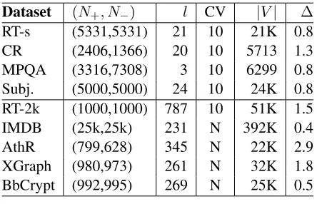
We compare with published results on the following datasets. Detailed statistics are shown in table 1.
RT-s: Short movie reviews dataset containing one sentence per review (Pang and Lee, 2005).
Dataset (N+, N−) l CV |V| ∆
RT-s (5331,5331) 21 10 21K 0.8 CR (2406,1366) 20 10 5713 1.3 MPQA (3316,7308) 3 10 6299 0.8 Subj. (5000,5000) 24 10 24K 0.8 RT-2k (1000,1000) 787 10 51K 1.5 IMDB (25k,25k) 231 N 392K 0.4 AthR (799,628) 345 N 22K 2.9 XGraph (980,973) 261 N 32K 1.8 BbCrypt (992,995) 269 N 25K 0.5
Table 1: Dataset statistics. (N+, N−): number of
positive and negative examples. l: average num-ber of words per example. CV: numnum-ber of cross-validation splits, or N for train/test split. |V|: the vocabulary size.∆: upper-bounds of the differences required to be statistically significant at thep <0.05 level.
CR: Customer review dataset (Hu and Liu, 2004) processed like in (Nakagawa et al., 2010).2 MPQA: Opinion polarity subtask of the MPQA
dataset (Wiebe et al., 2005).3
Subj: The subjectivity dataset with subjective re-views and objective plot summaries (Pang and Lee, 2004).
RT-2k: The standard 2000 full-length movie re-view dataset (Pang and Lee, 2004).
IMDB: A large movie review dataset with 50k full-length reviews (Maas et al., 2011).4
AthR, XGraph, BbCrypt: Classify pairs of newsgroups in the 20-newsgroups dataset with all headers stripped off (the third (18828) ver-sion5), namely: alt.atheism vs. religion.misc, comp.windows.x vs. comp.graphics, and rec.sport.baseball vs. sci.crypt, respectively.
4 Experiments and Results
4.1 Experimental setup
We use the provided tokenizations when they exist. If not, we split at spaces for unigrams, and we filter out anything that is not[A-Za-z]for bigrams. We do
2http://www.cs.uic.edu/∼liub/FBS/sentiment-analysis.html 3
http://www.cs.pitt.edu/mpqa/
4
http://ai.stanford.edu/∼amaas/data/sentiment 5
[image:2.612.315.537.62.205.2]not use stopwords, lexicons or other resources. All results reported useα = 1, C = 1, β = 0.25for NBSVM, andC= 0.1for SVM.
For comparison with other published results, we use either 10-fold cross-validation or train/test split depending on what is standard for the dataset. The CV column of table 1 specifies what is used. The standard splits are used when they are available. The approximate upper-bounds on the difference re-quired to be statistically significant at thep < 0.05 level are listed in table 1, column∆.
4.2 MNB is better at snippets
(Moilanen and Pulman, 2007) suggests that while “statistical methods” work well for datasets with hundreds of words in each example, they cannot handle snippets datasets and some rule-based sys-tem is necessary. Supporting this claim are examples such asnot an inhumane monster6, orkilling cancer
that express an overall positive sentiment with nega-tive words.
Some previous work on classifying snippets in-clude using pre-defined polarity reversing rules (Moilanen and Pulman, 2007), and learning com-plex models on parse trees such as in (Nakagawa et al., 2010) and (Socher et al., 2011). These works seem promising as they perform better than many sophisticated, rule-based methods used as baselines in (Nakagawa et al., 2010). However, we find that several NB/SVM variants in fact do better than these state-of-the-art methods, even compared to meth-ods that use lexicons, reversal rules, or unsupervised pretraining. The results are in table 2.
Our SVM-uni results are consistent with BoF-noDic and BoF-w/Rev used in (Nakagawa et al., 2010) and BoWSVM in (Pang and Lee, 2004). (Nakagawa et al., 2010) used a SVM with second-order polynomial kernel and additional features. With the only exception being MPQA, MNB per-formed better than SVM in all cases.7
Table 2 show that a linear SVM is a weak baseline for snippets. MNB (and NBSVM) are much better on sentiment snippet tasks, and usually better than other published results. Thus, we find the
hypothe-6
A positive example from the RT-s dataset.
7
We are unsure, but feel that MPQA may be less discrimi-native, since the documents are extremely short and all methods perform similarly.
Method RT-s MPQA CR Subj. MNB-uni 77.9 85.3 79.8 92.6 MNB-bi 79.0 86.3 80.0 93.6 SVM-uni 76.2 86.1 79.0 90.8 SVM-bi 77.7 86.7 80.8 91.7 NBSVM-uni 78.1 85.3 80.5 92.4 NBSVM-bi 79.4 86.3 81.8 93.2
RAE 76.8 85.7 – –
RAE-pretrain 77.7 86.4 – – Voting-w/Rev. 63.1 81.7 74.2 –
Rule 62.9 81.8 74.3 –
BoF-noDic. 75.7 81.8 79.3 – BoF-w/Rev. 76.4 84.1 81.4 – Tree-CRF 77.3 86.1 81.4 –
BoWSVM – – – 90.0
Table 2: Results for snippets datasets. Tree-CRF: (Nakagawa et al., 2010) RAE: Recursive Autoen-coders (Socher et al., 2011). RAE-pretrain: train on Wikipedia (Collobert and Weston, 2008). “Voting” and “Rule”: use a sentiment lexicon and hard-coded reversal rules. “w/Rev”: “the polarities of phrases which have odd numbers of reversal phrases in their ancestors”. The top 3 methods are inboldand the best is alsounderlined.
sis that rule-based systems have an edge for snippet datasets to be false. MNB is stronger for snippets than for longer documents. While (Ng and Jordan, 2002) showed that NB is better than SVM/logistic regression (LR) with few training cases, we show that MNB is also better with short documents. In contrast to their result that an SVM usually beats NB when it has more than 30–50 training cases, we show that MNB is still better on snippets even with relatively large training sets (9k cases).
4.3 SVM is better at full-length reviews
[image:3.612.318.535.64.267.2]Our results RT-2k IMDB Subj.
MNB-uni 83.45 83.55 92.58
MNB-bi 85.85 86.59 93.56
SVM-uni 86.25 86.95 90.84
SVM-bi 87.40 89.16 91.74
NBSVM-uni 87.80 88.29 92.40 NBSVM-bi 89.45 91.22 93.18 BoW (bnc) 85.45 87.8 87.77 BoW (b∆t0c) 85.8 88.23 85.65
LDA 66.7 67.42 66.65
Full+BoW 87.85 88.33 88.45 Full+Unlab’d+BoW 88.9 88.89 88.13
BoWSVM 87.15 – 90.00
Valence Shifter 86.2 – –
tf.∆idf 88.1 – –
Appr. Taxonomy 90.20 – –
WRRBM – 87.42 –
[image:4.612.74.300.65.308.2]WRRBM + BoW(bnc) – 89.23 –
Table 3: Results for long reviews (RT-2k and IMDB). The snippet dataset Subj. is also included for comparison. Results in rows 7-11 are from (Maas et al., 2011). BoW: linear SVM on bag of words features. bnc: binary, no idf, cosine nor-malization. ∆t0: smoothed delta idf. Full: the full model. Unlab’d: additional unlabeled data. BoWSVM: bag of words SVM used in (Pang and Lee, 2004).Valence Shifter: (Kennedy and Inkpen, 2006). tf.∆idf: (Martineau and Finin, 2009). Ap-praisal Taxonomy: (Whitelaw et al., 2005). WR-RBM: Word Representation Restricted Boltzmann Machine (Dahl et al., 2012).
ones that use additional data. These sentiment anal-ysis results are shown in table 3.
4.4 Benefits of bigrams depends on the task
Word bigram features are not that commonly used in text classification tasks (hence, the usual term, “bag of words”), probably due to their having mixed and overall limited utility in topical text classifica-tion tasks, as seen in table 4. This likely reflects that certain topic keywords are indicative alone. How-ever, in both tables 2 and 3, adding bigramsalways
improved the performance, and often gives better results than previously published.8 This presum-ably reflects that in sentiment classification there are
8
However, addingtrigramshurts slightly.
Method AthR XGraph BbCrypt
MNB-uni 85.0 90.0 99.3
MNB-bi 85.1 +0.1 91.2 +1.2 99.4 +0.1
SVM-uni 82.6 85.1 98.3
SVM-bi 83.7 +1.1 86.2 +0.9 97.7 −0.5
NBSVM-uni 87.9 91.2 99.7
NBSVM-bi 87.7 −0.2 90.7 −0.5 99.5 −0.2
ActiveSVM – 90 99
DiscLDA 83 – –
Table 4: On 3 20-newsgroup subtasks, we compare to DiscLDA (Lacoste-Julien et al., 2008) and Ac-tiveSVM (Schohn and Cohn, 2000).
much bigger gains from bigrams, because they can capture modified verbs and nouns.
4.5 NBSVM is a robust performer
NBSVM performs well on snippets and longer doc-uments, for sentiment, topic and subjectivity clas-sification, and is often better than previously pub-lished results. Therefore, NBSVM seems to be an appropriate and very strong baseline for sophisti-cated methods aiming to beat a bag of features.
One disadvantage of NBSVM is having the inter-polation parameterβ. The performance on longer documents is virtually identical (within 0.1%) for
β ∈[¼,1], whileβ = ¼ is on average 0.5% better for snippets thanβ = 1. Using β ∈ [¼,½]makes the NBSVM more robust than more extreme values.
4.6 Other results
Multivariate Bernoulli NB (BNB) usually performs worse than MNB. The only place where BNB is comparable to MNB is for snippet tasks using only unigrams. In general, BNB is less stable than MNB and performs up to 10% worse. Therefore, bench-marking against BNB is untrustworthy, cf. (McCal-lum and Nigam, 1998).
For MNB and NBSVM, using the binarized MNB
ˆfis slightly better (by 1%) than using the raw count
[image:4.612.316.540.65.187.2]References
R. Collobert and J. Weston. 2008. A unified architecture for natural language processing: Deep neural networks with multitask learning. InProceedings of ICML. George E. Dahl, Ryan P. Adams, and Hugo Larochelle.
2012. Training restricted boltzmann machines on word observations.arXiv:1202.5695v1 [cs.LG]. Rong-En Fan, Kai-Wei Chang, Cho-Jui Hsieh, Xiang-Rui
Wang, and Chih-Jen Lin. 2008. LIBLINEAR: A li-brary for large linear classification. Journal of Ma-chine Learning Research, 9:1871–1874, June. Minqing Hu and Bing Liu. 2004. Mining and
summariz-ing customer reviews. InProceedings ACM SIGKDD, pages 168–177.
Alistair Kennedy and Diana Inkpen. 2006. Sentiment classification of movie reviews using contextual va-lence shifters.Computational Intelligence, 22. Simon Lacoste-Julien, Fei Sha, and Michael I. Jordan.
2008. DiscLDA: Discriminative learning for dimen-sionality reduction and classification. InProceedings of NIPS, pages 897–904.
Andrew L. Maas, Raymond E. Daly, Peter T. Pham, Dan Huang, Andrew Y. Ng, and Christopher Potts. 2011. Learning word vectors for sentiment analysis. In Pro-ceedings of ACL.
Justin Martineau and Tim Finin. 2009. Delta tfidf: An improved feature space for sentiment analysis. In Pro-ceedings of ICWSM.
Andrew McCallum and Kamal Nigam. 1998. A compar-ison of event models for naive bayes text classification. InAAAI-98 Workshop, pages 41–48.
Vangelis Metsis, Ion Androutsopoulos, and Georgios Paliouras. 2006. Spam filtering with naive bayes -which naive bayes? InProceedings of CEAS.
Karo Moilanen and Stephen Pulman. 2007. Sentiment composition. InProceedings of RANLP, pages 378– 382, September 27-29.
Tetsuji Nakagawa, Kentaro Inui, and Sadao Kurohashi. 2010. Dependency tree-based sentiment classification using CRFs with hidden variables. InProceedings of ACL:HLT.
Andrew Y Ng and Michael I Jordan. 2002. On discrim-inative vs. generative classifiers: A comparison of lo-gistic regression and naive bayes. InProceedings of NIPS, volume 2, pages 841–848.
Bo Pang and Lillian Lee. 2004. A sentimental education: Sentiment analysis using subjectivity summarization based on minimum cuts. InProceedings of ACL. Bo Pang and Lillian Lee. 2005. Seeing stars: Exploiting
class relationships for sentiment categorization with respect to rating scales. InProceedings of ACL.
Jason D. Rennie, Lawrence Shih, Jaime Teevan, and David R. Karger. 2003. Tackling the poor assump-tions of naive bayes text classifiers. InProceedings of ICML, pages 616–623.
Greg Schohn and David Cohn. 2000. Less is more: Ac-tive learning with support vector machines. In Pro-ceedings of ICML, pages 839–846.
Richard Socher, Jeffrey Pennington, Eric H. Huang, An-drew Y. Ng, and Christopher D. Manning. 2011. Semi-Supervised Recursive Autoencoders for Pre-dicting Sentiment Distributions. In Proceedings of EMNLP.
Casey Whitelaw, Navendu Garg, and Shlomo Argamon. 2005. Using appraisal taxonomies for sentiment anal-ysis. InProceedings of CIKM-05.