The limits of central bank forward guidance under learning

Munich Personal RePEc Archive

The limits of central bank forward

guidance under learning

Cole, Stephen

Marquette University

22 March 2016

Online at

https://mpra.ub.uni-muenchen.de/70862/

The Limits of Central Bank Forward Guidance under

Learning

Stephen J. Cole ∗

March 22, 2016

Abstract

Central bank forward guidance emerged as a pertinent tool for monetary policymakers since the Great Recession. Nevertheless, the effects of forward guidance remain unclear. This paper investigates the effectiveness of forward guidance while relaxing two standard macroeconomic assumptions: rational expectations and frictionless financial markets. Agents forecast future macroeconomic variables via either the rational expectations hypothesis or a more plausible theory of expectations formation called adaptive learning. A standard Dynamic Stochastic General Equilibrium (DSGE) model is extended to include the financial accelerator mechanism. The results show that the addition of financial frictions amplifies the differences between ratio-nal expectations and adaptive learning to forward guidance. The macroeconomic variables are overall more responsive to forward guidance under rational expectations than under adaptive learning. During a period of economic crisis (e.g. a recession), output under rational expec-tations displays more favorable responses to forward guidance than under adaptive learning. These differences are exacerbated when compared to a similar analysis without financial fric-tions. Thus, monetary policymakers should consider the way in which expectations and credit frictions are modeled when examining the effects of forward guidance.

Keywords: Forward Guidance, Monetary Policy, Adaptive Learning, Expectations, Financial

Frictions.

JEL classification: D84, E30, E44, E50, E52, E58, E60.

∗_{I would like to thank Fabio Milani, William Branch, Eric Swanson, and Marco Del Negro for their very helpful}

comments and advice.

1

Introduction

The conventional monetary policy tool of lowering overnight interest rates was exhausted when the

zero lower bound (ZLB) on U.S. short-term nominal interest rates was effectively reached during

the 2007-2009 global financial crisis. Central banks around the world responded by pursuing

“un-conventional” monetary policies to stimulate their economies. One of these alternatives tools was

forward guidance where the central bank communicates to the public information about the future

path of the policy rate. For instance, the Federal Reserve issued forward guidance in the

Septem-ber 2012 Federal Open Market Committee (FOMC) statement: “the Committee also . . . anticipates

that exceptionally low levels for the federal funds rate are likely to be warranted at least through

mid-2015.” In addition, Eggertsson and Woodford (2003) and Woodford (2012) argue that

com-munication on the future path of interest rates can have stimulative economic effects. Standard

New Keynesian models (e.g. Woodford [2003]) predict agents being forward looking when making

current period decisions. If households and firms expect higher interest rates in response to future

expansions, economic activity today may be limited. However, if a central bank communicates a

low policy rate through part of the expansion, output today will not be as constrained.

The effectiveness of forward guidance hinges on two key channels–financial markets and

expectations–that are largely overlooked in standard macroeconomic models. The addition of credit

frictions in macroeconomic models is not a standard assumption. Frictionless financial markets are

largely assumed for simplicity and not to model realistic features of an economy. However, this

absence removes the prominent role of credit frictions in the macroeconomy and a key medium

through which forward guidance influences the economy. In addition, the way in which private

sector expectations about macroeconomic variables (e.g. output and inflation) respond to forward

guidance defines a key channel through which this unconventional monetary policy operates. The

standard way to model expectations in macroeconomic models is the rational expectations

hypoth-esis. However, this expectations formation scheme makes strong assumptions about the amount of

knowledge agents possess when constructing forecasts. Therefore, it is natural to investigate the

effectiveness of forward guidance when agents construct forecasts through a more realistic theory

of expectations formation.

This paper studies the effectiveness of forward guidance in an environment where credit

market frictions persist and rational expectations has been replaced by an adaptive learning rule

similar to one proposed by Marcet and Sargent (1989) and Evans and Honkapohja (2001). In

particular, the economic environment is based on the Federal Reserve Bank of New York-Dynamic

and Patterson (2012) and Del Negro et al. (2013). The model adds to a standard DSGE model

both financial frictions and central bank communication about the future path of interest rates.

A standard monetary policy rule is augmented with anticipated shocks as in Las´een and Svensson

(2011). The anticipated shocks represent future changes from a normal interest rate rule that

the central bank communicates to agents today. The shocks are also included to model

time-contingent forward guidance in which the central bank communicates to the public a forward

guidance completion date.

Agents are assumed to form expectations of future macroeconomic variables via two options:

the rational expectations hypothesis or a popular alternative called adaptive learning. Rational

expectations is a strong assumption. Agents form expectations based on the true model of the

economy as they know the model’s deep parameters, structure of the model, beliefs of other agents,

and distribution of the error terms. A popular alternative to rational expectations is adaptive

learning in which agents behave as real-life economists (see, for instance, Evans and Honkapohja

[2013]). Adaptive learning agents formulate forecasts of future endogenous variables by creating an

econometric model using variables based on the solution found under rational expectations. They

estimate the parameters of the model using ordinary least squares and appropriately adjust their

forecasts to new data each period.1

The inclusion of financial frictions follows Bernanke, Gertler, and Gilchrist (1999) and

Chris-tiano, Motto, and Rostagno (2009) and adds a realistic feature. The new components model the

borrowing and lending of funds seen in the real economy by adding two types of agents to a standard

medium scale DSGE model: banks and entrepreneurs. Banks take in deposits from households and

lend to entrepreneurs. The latter type of agents use these funds to purchase capital and rent it

to intermediate goods producers. Banks charge entrepreneurs a premium over the riskless

inter-est rate as there is a possibility they default. This “spread” fluctuates based on entrepreneurs’

leverage and an idiosyncratic shock that affects the perceived riskiness of entrepreneurs by banks.

If riskiness increases, entrepreneurs have a harder time receiving funds, and thus, are constrained

in the amount of capital they can funnel to the production side of the economy. The spread or

riskiness shock captures how the financial sector contributed to the Great Recession. Del Negro

et al. (2013) explain that spread shocks caused about half the decrease in U.S. output during the

Great Recession.

The results show that the addition of financial frictions amplifies the differences between

1

rational expectations and adaptive learning to forward guidance statements. These outcomes are

first shown under impulse responses of the macroeconomic variables to forward guidance shocks.

For instance, output’s response to forward guidance is stronger under rational expectations than

adaptive learning. Output displays a larger reaction to forward guidance under the former than

latter expectations formation scheme. The results are also presented during a period of economic

crisis (e.g. a recession). The central bank responds to the recession by communicating to the

public that the nominal interest rate will equal zero throughout the forward guidance horizon.

This exercise shows that the effects of forward guidance are overstated under rational expectations

relative to adaptive learning. Specifically, the value of output is higher under rational expectations

than adaptive learning throughout the forward guidance horizon. In addition, when the effect of

financial frictions in model is reduced, the “wedge” that existed between the responses of rational

expectations and adaptive learning to forward guidance diminishes. When compared to an analysis

without a financial sector included in the model (e.g. Cole [2015]), the differences between rational

expectations and adaptive learning in this present paper are also exacerbated. For instance, in

response to forward guidance announcements, the difference in output during an economic crisis is

larger between rational expectations and adaptive learning in this current paper than in a similar

analysis without financial frictions in Cole (2015).

The reasons for the differences arise from the amount of knowledge that agents are assumed

to hold and the additional financial variables to forecast. Under rational expectations, agents base

their expectations of future macroeconomic variables on the true model of the economy. Thus,

rational expectations agents compute precise expectations about how forward guidance statements

affect future macroeconomic variables. However, adaptive learning agents are not endowed with this

level of knowledge. Instead, they estimate the effects of forward guidance using their econometric

model of the economy. In addition, the inclusion of a financial sector magnifies the differences

be-tween rational expectations and adaptive learning agents. There exists more inertia in the adaptive

learning forecasting model and more variables to forecast than in a model without financial

fric-tions. These previous reasons and the fact that adaptive learning agents are estimating the effects

of forward guidance create bigger differences between the two types of expectations assumptions.

Overall, the results of the paper suggest a main finding for monetary policymakers: the

effects of forward guidance depend on the manner in which expectations and financial frictions are

modeled. Under the assumption of rational expectations, forward guidance produces more favorable

values of output than under adaptive learning. When including credit frictions, these differences

1.1 Previous Literature

This paper contributes to the growing literature on forward guidance. The seminal work by

Eg-gertsson and Woodford (2003) explains the importance of the expectations channel on the economy.

The path of short-term interest rates affect long-term interest rates and asset prices, and thus, the

management of interest rate expectations is pertinent for a central bank. McKay, Nakamura, and

Steinsson (2015) explain that the extreme responses of macroeconomic variables to forward

guid-ance found in standard macroeconomic models depend on the assumption of complete markets. The

addition of precautionary savings into a macroeconomic model limits the effectiveness of forward

guidance at the ZLB. The results from Del Negro et al. (2012) and Carlstrom, Fuerst, and

Paus-tian (2012) display unusually large responses of the macroeconomic variables to forward guidance

relative to the data. Del Negro et al. (2012) label this outcome “the forward guidance puzzle.”

This present paper suggests that the unusually large responses may be due to the rational

expecta-tions assumption employed in Del Negro et al. (2012), and a more realistic expectation formation

assumption (e.g. adaptive learning) produces results that better match the data.

The current paper follows recent literature examining the effectiveness of forward guidance.

De Graeve, Ilbas, and Wouters (2014) study the effects of forward guidance through a different lens

than the expectations channel. They find that the effects of this unconventional monetary policy

tool vary depending on the type of forward guidance and the underlying reasons for implementing

it (e.g. monetary stimulus or sign of future economic crisis). Levin, L´opez-Salido, Nelson, and

Yun (2010) explain that the power of forward guidance is sensitive to the type of structural shock

affecting the economy. Swanson and Williams (2014) show that Federal Reserve forward guidance

statements influence the economy by affecting medium- and longer-term interest rates. Kool and

Thornton (2012) test the effectiveness of forward guidance across four countries: New Zealand,

Norway, Sweden, and the United States. They find forward guidance helped market participants

forecast future short-term yields. In addition, Cole (2015) examines the effects of forward guidance

across rational expectations and adaptive learning assumptions, but utilizes a DSGE model without

financial frictions. The present paper shows that the differences between rational expectations and

adaptive learning to forward guidance are amplified when a DSGE model is expanded to include a

financial sector.

This paper fits into the literature on expectation formation and policy. Caputo, Medina, and

Soto (2010) use a DSGE model with adaptive learning and a financial accelerator as in Bernanke

et al. (1999). They find that the financial accelerator model with adaptive learning leads to large

volatility in output and inflation. When the fiscal authority communicates information about the

future path of government purchases and taxes, Mitra, Evans, and Honkapohja (2012) show that

output multipliers match the data more under adaptive learning than rational expectations. Eusepi

and Preston (2010) examine the benefits of central bank communication in which agents have an

incomplete model of the economy when constructing expectations. When a central bank provides

more information to the public about policy (e.g. the variables within a monetary policy rule),

the macroeconomic variables exhibit greater stability as agents are able to construct more precise

forecasts. Woodford (2010) studies optimal monetary policy in which the central bank understands

agents may not form forecasts via the rational expectations hypothesis. He stresses the importance

of policy commitment (e.g. guaranteeing stable inflation) regardless of agents’ expectations not

being model consistent. Slobodyan and Wouters (2011) examine the medium-scale DSGE model of

Smets and Wouters (2007) under the assumption of adaptive learning. The DSGE model’s match

to the data is on par or exceeds the results under adaptive learning than rational expectations.

The remaining sections are organized as follows. Section two presents the DSGE model with

financial frictions. Section three discusses expectations formation under both rational expectations

and adaptive learning. Section four contains the results of forward guidance under both types of

expectations formations. Impulse response functions, forward guidance during an economic crisis,

and the importance of financial frictions for forward guidance are examined. The results are also

studied when the degree in which adaptive learning agents discount previous observations is varied.

Section five concludes.

2

Model

The aggregate dynamics of the economy are described by a medium scale DSGE model with financial

frictions following Del Negro et al. (2012) and Del Negro et al. (2013). It contains a large number

of frictions found in standard DSGE models (e.g. Smets and Wouters [2007]). These include price

and wage stickiness, price and wage indexation, habit formation in consumption, capital utilization,

and investment adjustment costs. The model also includes credit frictions following Bernanke et

al. (1999) and Christiano et al. (2009). The remainder of this section presents a brief description

of the model followed by the log-linearized equations.

2.1 Description

Households and Labor Packers: Each household j ∈[0,1] maximizes the sum of its expected

firms. A household supplies its work to labor packers (e.g. employment agencies). The latter

group bundles labor to sell to intermediate goods producers in a perfectly competitive market. In

addition, a household can put its wealth in government issued bonds, deposits held at banks, and

money. As will be discussed later, the deposits held at banks are important as entrepreneurs use

it to purchase capital. The entrepreneurs funnel capital to the production side of the economy.

The frictions in the household sector take the form of habit formation in consumption and

wage stickiness. Households have market power in the labor market and choose their nominal

wage subject to the amount of work demanded by intermediate goods producers. Following Calvo

(1983), a household has probability (1−ζ_w) of choosing its wage each period, and a probabilityζ_w

of not being able to choose its wage. Under the latter scenario, wages are indexed to either previous

period’s inflation times last period’s productivity with probabilityιw, or steady state inflation times

the economy’s growth rate with probability (1−_ιw).

Firms: There exist two types of firms: intermediate and final goods producers. Intermediate

goods producers operate in a monopolistically competitive market and use labor and capital to

create differentiated products to sell to final goods producers. The source of their labor and

capital comes from households (via employment agencies) and entrepreneurs, respectively. The

intermediate goods producers are subject to nominal price rigidities in the form of a Calvo (1983)

pricing scheme. In each period, firms have a probability (1−ζ_p) of freely changing their price. The

remaining fractionζp of firms index their price to either previous period’s inflation with probability

ιp or the steady state rate of inflation with probability (1−ιp). The final goods producers conduct

business in a competitive market and bundle the intermediate goods into one composite good.

Financial Sector and Capital Producers: The modeling of credit frictions starts with

two agents: banks and entrepreneurs. Banks pay interest on deposits received from households and

use the funds to issue loans to entrepreneurs. The entrepreneurs use the funds to purchase capital

from capital producers and rent it to intermediate goods firms. Banks also charge entrepreneurs

a premium over the risk-free interest rate as there is a risk of default. This “spread” varies with

entrepreneurs’ leverage, that is, the ratio of the value of capital to net worth. The spread widens

as the value of entrepreneurs’ capital, which is positively related to the amount it borrows from

banks, increases relative to its own net worth. In every period, an idiosyncratic shock also affects the

amount of capital that entrepreneurs manage. An adverse shock shrinks the amount of capital they

can lend, and thus, the proceeds they earn from lending to intermediate goods firms. Consequently,

this negative shock decreases the ability of entrepreneurs to repay their loans to the bank. In

can reflect entrepreneurs’ perceived riskiness by banks to repay loans. If the riskiness increases,

banks will increase the amount it charges entrepreneurs for loans. As the cost of borrowing rises,

the ability of entrepreneurs to buy capital to rent to intermediate goods producers diminishes.

Capital producers operate in a perfectly competitive market and are responsible for the

creation of the stock of capital. They purchase a part of output from final goods producers and

transform it into capital subject to adjustment costs. They also purchase a fraction of capital

from entrepreneurs. These two sources of capital comprise the amount of capital for use next

period. Capital producers sell capital back to entrepreneurs who then rent it to intermediate goods

producers.

Government Policy: The model includes both monetary and fiscal policies. The monetary

authorities follow a Taylor-type rule and adjust the short-term nominal interest rate to changes in

output, inflation, monetary policy shock, and anticipated or forward guidance shocks. The fiscal

authorities collect lump-sum taxes and satisfy a government budget constraint. There also exists

a government spending shock which captures exogenous fluctuations in aggregate demand.

2.2 Log-linearized Equations

The following are the set of log-linearized equations that describe the DSGE model with financial

frictions. The “ ˆ ” and “ * ” symbols represent log deviations from steady state and steady state

values, respectively. The ˆEt indicates (potentially) non-rational expectations, whileEt denotes the

model-consistent rational expectations operator. From the household’s first-order conditions, one

can get the consumption Euler equation:

ˆ

ξt= ˆRt+ ˆEtξˆt+1−Eˆtπˆt+1 (1)

where ˆξtis the marginal utility of consumption, ˆRt is the nominal interest rate paid on government

issued bonds and controlled by the central bank, and ˆπt is the inflation rate. Consumption is

defined according to the following equation:

(eγ−hβ)(eγ−h) ˆξ_t=eγ(eγ−h)ˆb_t−(e2γ+βh2)ˆc_t+heγcˆ_t

−1

−βh(eγ−h) ˆE_tˆb_t+1+βheγEˆ_tˆc_t+1

(2)

where ˆct is consumption, ˆbt is a stochastic shock to household utility, β is the discount factor, h

represents habit formation in consumption, and eγ _{is the steady-state (gross) growth rate of the}

economy. The demand for money by households is given by

vmmˆt=−

1

R∗−1

ˆ

where ˆmtis money.

Households have market power in the labor market. Wages are chosen by households

accord-ing to a Calvo (1983) scheme. In each period, a fraction 1−_ζw of households can choose their

wage. The remaining ζw of households index wages to either previous period’s inflation times last

period’s productivity with probabilityιw, or steady state inflation times the economy’s growth rate

with probability (1−ι_w). The optimal reset wage equation is given by

(1 +νl

1 +λw

λw

) ˆw˜t+ (1 +ζwβνl(

1 +λw

λw

)) ˆwt=ζwβ(1 +νl

1 +λw

λw

) ˆEt( ˆw˜t+1+ ˆwt+1)

+ (1−_ζwβ)(_e2γ+_h2_β) e

−γ

eγ_−hˆbt+ ˆϕt+ (1−ζwβ)(νlLˆt−ξˆt)

−_ζwβιw(1 +_νl1 +λw

λw

)ˆπt+ζwβ(1 +νl

1 +λw

λw

) ˆEtπˆt+1

(4)

ˆ ˜

wtrepresents the freely chosen wage by households, ˆwtis the aggregate wage, ˆLtis aggregate labor,

and ˆϕt is a stochastic shock that affects the marginal utility of labor. λw defines the elasticity of

substitution between differentiated labor services, andνl represents the inverse Frisch elasticity of

labor supply. In addition, the aggregate wage equation is given by

ˆ

wt= ˆwt−1+ιwπˆt−1−πˆt+

1−_ζw

ζw

ˆ ˜

wt (5)

The production side of the economy is populated by intermediate and final goods producing

firms. The intermediate goods firms operate in a monopolistically competitive market while final

goods producers conduct business in a competitive market. Prices do not freely adjust in the

former market. Specifically, a fraction (1−_ζp) of firms can freely adjust its price every period. The

remainingζp of firms either index prices to previous period’s inflation with probabilityιp or steady

state rate of inflation with probability (1−ι_p). Consequently, the Phillips Curve is given by

ˆ

πt=

ιpζp

1 +ιpβ

ˆ

πt−1+

β

1 +ιpβ

ˆ

Etπˆt+1+

(1−_ζpβ)(1−_ζp)

(1 +ιpβ)ζp

ˆ

mct+

1

(1 +ιpβ)ζp

ˆ

λf,t (6)

where ˆλf,t represents a cost-push shock. ˆmct is marginal cost and is defined by

ˆ

mct= (1−α) ˆw_t+αrˆ_tk (7)

where ˆrk_t is the rental rate of capital andα captures capital’s share of output. Intermediate goods

firms utilize both labor and capital in a Cobb-Douglas production function given by

ˆ

yt=

α(y∗_{+ Φ)}

y∗

ˆ

kt+

(1−α)(y∗+ Φ)

y∗

ˆ

Lt (8)

The model’s resource constraint satisfies

ˆ

yt= ˆgt+

c∗

c∗+i∗ˆct+

i∗

c∗+i∗

ˆ_it+ rk∗k∗

c∗+i∗uˆt (9)

where ˆit is investment, ˆut is capital utilization, and ˆgt is a government spending shock capturing

exogenous aggregate demand fluctuations in the economy.

The capital-to-labor ratio is given by

ˆ

kt= ˆwt−rˆkt + ˆLt (10)

The financial side of the economy is populated by banks and entrepreneurs. Entrepreneurs

borrow funds from banks to purchase capital from capital producers and rent it to intermediate

goods producers. The amount of funds entrepreneurs can borrow is a function of their net worth,

which evolves according to the following equation:

ˆ

nt=ζ_n,R˜k( ˆR˜

k

t −πˆt)−ζn,R( ˆRt−1−πˆt) +ζn,qK(ˆqkt−1+ ˆk¯t−1)

+ζn,nnˆt−1+ ˆγt−

ζn,µe

ζsp,µeµˆ

e t−1−

ζn,σω

ζsp,σω

ˆ

σω,t−1

(11)

where ˆq_tk is the price of capital, ˆ¯kt measures the amount of installed capital, ˆγt defines the

time-varying exogenous fraction of entrepreneurs that survive each period shock, ˆµe

t is a bankruptcy cost

shock, and ˆσω,t is a spread shock. ζ_n,R˜k, ζn,R, ζn,qK, ζn,n, ζn,µe,and ζ_n,σ

ω are the elasticities of net

worth with respect to the return on capital, nominal interest rate, price of capital, net worth itself,

bankruptcy cost shock, and the spread shock, respectively. ζsp,σω represents the elasticity of the

spread with respect to the volatility of the spread shock. ζsp,µe is the elasticity of the spread with

respect to the bankruptcy cost shock. ˆR˜_tk is the gross return on capital entrepreneurs receive from

renting capital to intermediate goods producers and is defined by

ˆ ˜

Rk_t −πˆ_t= r k

∗

rk

∗+ (1−δ)

ˆ

rk_t + 1−δ

rk

∗ + (1−δ)

ˆ

q_tk−qˆk_t

−1 (12)

whereδ is the depreciation rate. The expected excess return on capital or spread is defined by the

following equation

ˆ

Et( ˆR˜kt+1−Rˆt) =ζsp,b(ˆqtk+ ˆk¯t−nˆt) + ˆµet + ˆσω,t (13)

where ˆσω,t is defined as a spread shock. It characterizes banks’ perception of the riskiness of

entrepreneurs. For example, if this shock increases, banks perceive entrepreneurs to be risky and

thus, bank loans are harder to receive. This decrease in funds hampers the ability of entrepreneurs

entrepreneurs’ leverage, which is defined as the ratio of the value of capital to nominal net worth.

The amount of installed capital in the model is given by

ˆ ¯

kt= (1−

i∗

k∗)ˆ

¯

kt−1+

i∗

k∗µˆt+

i∗

k∗

ˆ_{it (14)}

where ˆµt is a shock to the amount of capital. The amount of investment ˆit is defined by

ˆ_it= 1

1 +βˆit−1+

β

1 +βEˆtˆit+1+

1

(1 +β)S′′

e2γqˆ k

t + ˆµt (15)

whereS(•) captures the cost of adjusting capital and S′ >0 and S′′>0.

The amount of capital is described by the following equation:

ˆ

kt= ˆut+ ˆk¯t−1 (16)

ˆ

ut defines the capital utilization rate and the corresponding equation is given by

r_∗krˆk_t =a′′uˆt (17)

wherea′′ captures capital utilization costs.

Monetary Policy: The model’s central bank adjusts the short-term nominal interest rate

using the following monetary policy rule:

ˆ

Rt=ψππˆt+ψyyˆt+εM Pt + L

X

l=1

εR_l,t−l (18)

where εM P_t defines an unanticipated monetary policy shock. Forward guidance is added into the

model by augmenting the monetary policy rule with anticipated shocks similar to Del Negro et al.

(2012), Las´een and Svensson (2011), and Cole (2015). Each anticipated or forward guidance shock

(εR_l,t−l) is contained in the termP_lL=1εRl,t−l found in equation (18) and isi.i.d.

2

A forward guidance

shock defines a central bank announcement in periodt−lthat the interest rate will changelperiods

later, that is, in periodt. In addition,Lrepresents the length of the central bank’s time-contingent

forward guidance horizon. Thus, there are Lforward guidance shocks in equation (18) that affect

the monetary policy rule in period t. Following Del Negro et al. (2012) and Las´een and Svensson

(2011), the system is also augmented with L state variablesv1,t, v2,t, ..., vL,t whose laws of motion

2

is given by

v1,t = v2,t−1+εR_1,t (19)

v2,t = v3,t−1+εR2,t (20)

v3,t = v4,t−1+εR3,t (21)

.. .

vL,t = εRL,t (22)

Each term invt= [v1,t, v2,t, ..., vL,t]′ contains the sum of all forward guidance statements known to

agents in periodtthat change the interest rate 1,2, ...,andLperiods later, respectively. Equations

(19)−(22) can also be simplified to find that v_1,t−1 =PL

l=1εRl,t−l, which is the sum of all forward

guidance commitments announced by the central bank 1,2, ..., and L periods ago that affect the

interest rate in period t. In addition, the main reason to model forward guidance in this manner

regards indeterminacy. If forward guidance is alternatively modeled as pegging the interest rate

to a certain value, indeterminacy can arise as described in Honkapohja and Mitra (2005) and

Woodford (2005). For instance, without a monetary policy that responds to economic activity,

real disturbances to the economy can produce multiple equilibria.3 _{However, forward guidance}

modeled by equations (19)−(22) can still attain a constant interest rate path. As will be described

in Section 4.3, the forward guidance shocks can be chosen such that the ˆRt = ¯R throughout the

forward guidance horizon.

The following example is provided to gain intuition on equations (19)-(22). Consider the case

in which the central bank’s forward guidance horizon is 2 periods ahead, i.e. L= 2. The model’s

system of equations includesv1,t andv2,t whose laws of motion are defined as

v1,t = v2,t−1+εR1,t =εR2,t−1+εR1,t (23)

v2,t = εR2,t (24)

The variable vR

1,t contains all central bank forward guidance known in period t that affects the

interest rate one period later, that is,εR

2,t−1andεR1,t. Forward guidance known in periodtthat affects

the interest rate two periods later is defined by v2,t. This variable consists ofεR2,t, which is defined

as current period forward guidance that affects the interest rate two periods later. Furthermore,

the “ ˆ ” symbol over the variables is removed for the remainder of the paper to simplify notation.

3

2.3 Exogenous Shocks

The model’s exogenous shocks consist of a spread shock (σw,t), price mark-up shock (λf,t),

la-bor shock (ϕt), stochastic preference shock (bt), government spending shock (gt), marginal

ef-ficiency of investment shock (µt), bankruptcy cost shock (µet), time-varying exogenous survival

rate of entrepreneurs shock (γt), monetary policy shock (εM Pt ), and forward guidance shocks

(εR_1,t, εR_2,t, . . . , εR_L,t). Except for the unanticipated monetary policy and forward guidance shocks, the

structural shocks follow an AR(1) process with autocorrelation parameters (ρσw, ρλf, ρϕ, ρb, ρg, ρµ,

ρµe,and ρ_γ).

3

Expectations Formation

This paper assumes agents evaluate the expectations in equations (1)−(17) following either the

rational expectations hypothesis or adaptive learning. Rational expectations agents form

expecta-tions based on the true model of the economy. They know the structure of the model, parameters

of the model (e.g. ζp,h, etc.), distribution of the error terms, and beliefs of other agents. Adaptive

learning agents do not know the true model of the economy. Instead, they operate as real-life

economists (e.g. econometricians) by creating an econometric model of the economy to produce

forecasts of future economic variables. They estimate the parameters using standard econometric

techniques and revise their forecasts as new data arrives.4

Rational Expectations–The model under rational expectations is solved using standard

techniques (e.g. Sims [2002]). The model is written in general state-space form:

e

Γ0Yet=C+Γe1Yet−1+eΓ2εet+eΓ3ζt (25)

where

e

Yt = [Yt, ǫt, vt,Ξt]

′

(26)

Yt = [ξt, Rt, ct,¯kt, it, kt, ut, rkt, qt,R˜Kt , πt, nt, wt,w˜t, Lt, mct, yt, mt]

′

(27)

ǫt = [λf,t, µt, ϕt, gt, σw,t, bt, µet, γt]

′

(28)

vt = [v1,t, v2,t, . . . , vL,t]

′

(29)

Ξt = [Etξt+1, Etπt+1, Etct+1, Etit+1, EtR˜kt+1, Etw˜t+1, Etwt+1]

′

(30)

e

εt = [ελt, ε µ t, ε

ϕ t, ε

g t, ε

σw

t , εbt, ε µe

t , ε γ

t, εM Pt , εR1,t, εR2,t, . . . , εRL,t]

′

(31)

4

C denotes a vector of constants of required dimensions, Ytdefines a vector containing the model’s

endogenous variables, ǫt is a vector of the model’s exogenous processes, and Ξt denotes the vector

of expectations. The i.i.d. structural disturbances and forward guidance shocks are contained in

the vector εet. The expectational errors (e.g. ζtπ = πt−Et−1πt) are contained in the vector ζt of

required dimensions. When using the technique proposed by Sims (2002) and the parameter values

in Table 1 in Appendix A, the solution under rational expectations is

e

Yt=Ce+ξ1Yet−1+ξ2εet (32)

where the matricesCe,ξ1, and ξ2 are nonlinear functions of the model’s parameters.5

Adaptive Learning–Adaptive learning agents evaluate the expectations in equations (1)−

(17) by forming an econometric model and estimating the coefficients. This model is called the

“Perceived Law of Motion” (PLM) and contains the variables that appear in the minimum state

variable (MSV) solution that exists under rational expectations.6

The PLM is given by

Yt=a+bYt−1+cvt+d˜¯ǫt+ev1,t−1+εt (33)

where ˜ǫ¯t= [ǫt, εM Pt ]

′

. Yt,vt, and ǫt are defined as in the rational expectations model. In addition,

the reader should note thatvt ande¯ǫt can be expressed as

vt = Φvt−1+ηt (34)

˜ ¯

ǫt = φe˜¯ǫt−1+ ¯ǫt (35)

where Φ is an LxL matrix given by

Φ =

          

0 1 0 0 . . . 0 0

0 0 1 0 . . . 0 0

0 0 0 1 . . . 0 0

..

. . .. ...

0 0 0 0 . . . 1 0

0 0 0 0 . . . 0 1

0 0 0 0 . . . 0 0

          

(36)

5

Section 4.1 contains a discussion of the model’s parameter values.

6

and

ηt = [εR1,t, εR1,t, . . . , εRL,t]

′ (37) e φ =              

ρλf 0 0 0 0 0 0 0 0

0 ρµ 0 0 0 0 0 0 0

0 0 ρϕ 0 0 0 0 0 0

0 0 0 ρg 0 0 0 0 0

0 0 0 0 ρσw 0 0 0 0

0 0 0 0 0 ρb 0 0 0

0 0 0 0 0 0 ρµe 0 0

0 0 0 0 0 0 0 ργ 0

0 0 0 0 0 0 0 0 0

              (38) ¯

ǫt = [ελt, ε µ t, ε

ϕ t, ε

g

t, εwt , εbt, ε µe

t , ε γ t, εM Pt ]

′

(39)

a,b,c,d, andeare unknown coefficient matrices of appropriate dimensions that adaptive learning

agents estimate each period. The time subscript is not added to the PLM coefficients to highlight

that adaptive learning agents believe their expectations to be optimal every period. They do not

take into account they will be updating their beliefs in the future. However, the coefficients in the

PLM will evolve each period as will be described later. Furthermore, the addition of v1,t−1 in the

PLM is necessary. v1,t−1 is contained in the rational expectations solution but not found in the

vectorvt as seen in equations (34) and (36).

This paper assumes the following time line of events for the learning expectations formation

process:

1. At the beginning of period t, adaptive learning agents observe vt, and ˜¯ǫt and add these

variables to their information set.

2. Agents use previous period’s estimates (i.e. at−1,bt−1,ct−1,dt−1, and et−1) and Yt−1,vt, ˜ǫ¯t,

and v1,t−1 to construct forecasts of future endogenous variables.

3. The values of the endogenous variables contained in Yt are realized.

4. Adaptive learning agents update their parameter estimates by computing a least squares

regression ofYt on 1,Yt−1,vt, ˜¯ǫt, and v1,t−1.

Agents update their parameter estimates of the PLM by following the recursive least squares

(RLS) formula

φt = φt−1+τtRt−1zt(Yt−φ′_t

−1zt)′ (40)

Rt = Rt−1+τt(ztz

′

whereφ= (a, b, c, d, e)′ contains the PLM coefficients to be estimated andzt≡[1, Y_t−1, v_t,˜¯ǫ_t, v_1,t−1]′

defines the regressors in the PLM.Rtis the precision matrix of the regressors in the PLM. Adaptive

learning agents’ recent prediction error is given by the last expression in (40). The “gain” parameter

τt governs the degree in which φtresponds to new information.

This current paper examines the discounted or constant gain learning (CGL) case in which

the gain parameter is fixed to a certain value, that is,τt= ¯τ. As described in Evans and Honkapohja

(2001), the coefficients will converge in distribution to their rational expectations counterparts with

a variance proportional to τt = ¯τ. Under this scheme, recent observations also play a larger role

when adaptive learning agents are updating their coefficients. This assumption allows agents to

update their beliefs every period to new information (e.g. forward guidance) as is similar to real-life

economists updating their forecasts as new data arrive.7

Adaptive learning agents solve for ˆEtYt+1 by using equation (33). Specifically, expectations

are given by

ˆ

EtYt+1 = (I18+bt−1)at−1+b2_t−1Yt−1+ (bt−1ct−1+ct−1Φ)vt

+ (bt−1dt−1+dt−1φe)˜¯ǫt+bt−1et−1v1,t−1+et−1v1,t (42)

Equation (42) is substituted into equations (1)−(17) to give the “Actual Law of Motion” (ALM):

Yt= Γ0(φt−1) + Γ1(φt−1)Yt−1+ Γ2(φt−1)vt+ Γ3(φt−1)vt−1+ Γ4(φt−1)˜¯ǫt+ Γ5(φt−1)˜¯ǫt−1 (43)

The previous equation describes the evolution of the model’s endogenous variables implied by the

PLM in (33).

4

Results

4.1 Parameterization

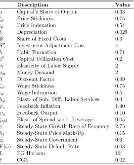
Table 1 in Appendix A displays the values of the parameters used in simulation. The values largely

follow from empirical work by Del Negro et al. (2012) and Del Negro et al. (2013). There exists a

high degree of habit formation in consumption withh= 0.71. a′′ = 0.2 indicates a smaller reaction

of the rental rate of capital to changes in the capital utilization rate. The value of the price

stickiness parameter implies that prices change once a year, which also corresponds to empirical

work by Klenow and Malin (2011). The inclusion of a financial sector also adds additional credit

7

This approach is in contrast to the decreasing gain or RLS case in whichτ_{t =}t−1

market parameters. The survival rate of entrepreneurs is set to 0.99. ζsp,b defines the elasticity of

the spread (Et( ˜RKt+1−Rt)) with respect to leverage (qtk+ ¯kt−nt) and equals to 0.05. For simplicity,

the structural shocks are assumed to be i.i.d. The distribution of the noise shocks is not assumed

to be highly dispersed. There also is no covariance between the structural shocks.

This current paper uses the CGL model as described in Section 3. The CGL parameter, ¯τ, is

chosen to be 0.02. This value closely follows Orphanides and Williams (2005), Milani (2007), and

Branch and Evans (2006).

The values of the monetary policy parameters in Table 1 closely match the existing literature.

Monetary policy positively responds to output and positively adjusts at more than a one-to-one rate

to inflation. The value ofχx closely follows Gilchrist, Ortiz, and Zakrajˇsek (2009) who estimated a

medium-scale DSGE model with financial frictions. The value of the inflation feedback parameter

(i.e. χπ) closely follows empirical adaptive learning work by Milani (2007). In addition,Lrepresents

the length of central bank time-contingent forward guidance and is set equal to 12. This number

is based off the FOMC September 2012 statement, which was one of its last announcements to

exclusively use time-contingent forward guidance language. In this statement, the FOMC said “the

Committee also decided today to keep the target range for the federal funds rate at 0 to 1/4 percent

and currently anticipates that exceptionally low levels for the federal funds rate are likely to be

warranted at least through mid-2015.” The number of quarters from September 2012 to “mid-2015”

is twelve when taking “mid-2015” to be at most the end of the third quarter of 2015.

4.2 Normal Economics Times

I first examine the differences between rational expectations and adaptive learning to forward

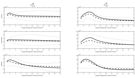
guidance under the DSGE model with financial frictions. K-period impulse responses of output,

investment, and inflation to negative one standard deviation forward guidance shocks under different

expectations assumptions are examined in Figures 1 and 2.8

In addition, adaptive learning impulse

response functions cannot be computed using standard linear techniques as equation (43) exhibits

a nonlinear structure. Thus, the following approach from Eusepi and Preston (2011) is utilized.

The model is simulated twice forT+ 1 +K periods whereK is the impulse response horizon and is

chosen to be twenty periods.9

One simulation contains a negative one standard deviation forward

guidance shock in periodT+ 1. The impulse responses are given by the difference between the two

simulations over the final K = 20 periods. This process is repeated a large number of times and

8

The forward guidance shocks are found in equations (19) - (22).

9

the average is taken to arrive at the reported impulse response function. Furthermore, the solid

lines in Figures 1 and 2 represent rational expectations impulse response functions. The dashed

lines denote the adaptive learning impulse response functions with 95% confidence bands given by

the dotted lines.10

Figures 1 and 2 show that the macroeconomic variables overall display a stronger reaction

to forward guidance under rational expectations than adaptive learning. Even though forward

guidance has stimulative effects on both expectations assumptions, the adaptive learning output

path exhibits a smaller reaction to forward guidance shocks than rational expectations. Rational

expectations agents’ forecasts are based on the true model of the economy. Consequently,

ratio-nal expectations agents understand the effects that statements about the future interest rate have

on future macroeconomic variables. However, adaptive learning agents are unable to base their

expectations on the true model of the economy as they are not endowed with that knowledge.

In-stead, they estimate the effects of forward guidance utilizing an econometric model of the economy.

Adaptive learning agents are continually adjusting their forecasts each period causing a smaller

reaction to forward guidance. In addition, the inclusion of a financial sector contributes to the

differences between adaptive learning and rational expectations. The financial sector produces

ad-ditional variables to forecast and more inertial behavior (lagged variables) in the PLM relative to a

model without financial frictions (e.g. Cole [2015]). Therefore, adaptive learning agents are slower

to understand the positive effects of forward guidance on the economy.

Overall, the message from this section is that rational expectations exhibits a stronger

reac-tion to forward guidance and a financial sector compounds the differences between the two types

of agents. When the central bank communicates forward guidance to agents, the adaptive learning

path of output is different than rational expectations. Rational expectations agents precisely

un-derstand the effects forward guidance has on macroeconomic variables as they base their beliefs on

the true model of the economy. However, the expectations of adaptive learning agents are slower

to adjust to forward guidance statements as they base their forecasts on an estimated model of the

economy. The presence of financial frictions also creates a slower response of adaptive learning to

forward guidance than rational expectations.

4.3 Economic Crisis

Central bank forward guidance was implemented in response to the 2007-2009 financial crisis. With

that event in mind, this section examines the effects of forward guidance during a period of

eco-10

nomic crisis (e.g. a recession) under both rational expectations and adaptive learning assumptions.

Specifically, the central bank communicates forward guidance information such that the interest

rate ¯R = 0 throughout the recession and forward guidance horizon. The policy simulation is

described next and is motivated by similar exercises in Cole (2015) and Del Negro et al. (2012).

The model is first simulated until periodT+ 1. This time frame reflects a period of economic

stability (e.g. the period before the Great Recession). In periodT + 1, the economy experiences a

recession that lasts six periods.11 _{A large negative spread shock impacts the model in periodT+ 1}

followed by a sequence of five more adverse spread shocks.12 _{To counter the adverse effects in the}

economy, the central bank implements forward guidance. It communicates to the public that the

interest rate will equal ¯R= 0 in period T+ 1 andLperiods into the future. This forward guidance

announcement corresponds to an unanticipated change in the interest rate in period T + 1 and

anticipated changes in the interest rate in periodsT+ 2 throughT+L+ 1. Specifically, the central

bank chooses the unanticipated monetary policy shock,εM P

T+1, and the anticipated forward guidance

shocksηT+1= [εR_1,T+1, εR_2,T+1, . . . , εR_L,T+1] such that the nominal interest rate equals 0 from the time

periodT+1 throughT+L+1. In addition, the length of the central bank’s forward guidance spans

a recession and normal times sinceL= 12. If agents expect the interest rate to be lower than usual

even during economic expansions, that is, normal times, forward guidance can have additional

stimulative effects. The central bank also assumes that agents form their expectations via the

rational expectations hypothesis. This expectations formation scheme is the standard assumption

in macroeconomic models. The same forward guidance is then given to adaptive learning agents in

order to examine the differences between the two types of expectations formation assumptions.

The previously described exercise assumes that the central bank is committed to keeping

the interest rate at zero throughout the forward guidance horizon. Rational expectations agents

precisely understand how the central bank’s forward guidance statements affect the economy. Thus,

the interest rate equals ¯R= 0 throughout the forward guidance horizon. However, adaptive learning

agents have an incomplete model of the economy when forming expectations. By giving adaptive

learning agents the same forward guidance information that was given to rational expectations

agents, the interest rate will not achieve a model implied ¯R= 0 throughout the forward guidance

horizon. To model the central bank promising to keep ¯R = 0 over the forward guidance horizon

and ensure the interest rate is the same value in both rational expectations and adaptive learning,

this policy exercise follows Cole (2015) such that the central bank chooses εM P

t each period to

11

The recession’s length is chosen in accordance with the National Bureau of Economic Research’s definition of the 2007-2009 Great Recession.

12

guarantee that ¯R= 0.

The spread shock operates through the financial sector to cause a downturn in the economy. A

higher spread implies banks perceive entrepreneurs to be riskier, and thus, borrowing costs and cost

of capital for firms increase. This result hinders firms from receiving capital from entrepreneurs.

Lower economic activity results from less capital being channeled to the production side of the

economy. Furthermore, the modeling of a recession via a spread shock closely matches the data.

Del Negro et al. (2013) show that spread shocks accounted for about half the decline in output

growth during the Great Recession in the U.S.

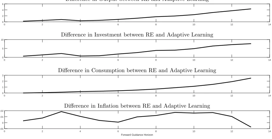
Figure 3 displays the macroeconomic effects of forward guidance during an economic

reces-sion. The difference between rational expectations and adaptive learning of different macroeconomic

variables is plotted. A positive value indicates the macroeconomic variable’s value is higher under

rational expectations than adaptive learning. If the value is negative, the value of the

macroeco-nomic variable is lower under rational expectations than adaptive learning. The figure shows that

the stimulative economic effects of forward guidance are overstated under rational expectations

than adaptive learning. Specifically, the value of output in the top panel of Figure 3 is higher under

rational expectations than adaptive learning across the entire forward guidance horizon.

What accounts for the higher response of output to forward guidance under rational

expecta-tions than adaptive learning? The first source comes from the financial sector of the model. In the

bottom three panels of Figure 3, differences occur between the responses of rational expectations

and adaptive learning to forward guidance. However, the disparity is greater under investment

than consumption and inflation indicating that financial elements are driving the disparity in

out-put between rational expectations and adaptive learning. The differences between the amount of

the knowledge rational expectations and adaptive learning agents have about the economy also

influence the results seen in Figure 3. Since they construct forecasts using the true model of the

economy, rational expectations agents precisely understand how central bank forward guidance will

stimulate the economy. However, adaptive learning agents do not know the true model of the

economy when constructing their expectations. Since they use an econometric model to build their

forecasts, adaptive learning agentsestimate the effects of forward guidance on the economy. Thus,

they fail to understand all of the positive benefits of forward guidance.

The results in this section also relate to the “the forward guidance puzzle” found in Del Negro

et al. (2012). Their paper showed that central bank forward guidance produced an exceedingly

large reaction of the macroeconomic variables in relation to the data. Del Negro et al. (2012) also

paper is based on the model in Del Negro et al. (2012), but is solved under both the assumptions

of rational expectations and adaptive learning. As shown in the top panel of Figure 3, the value

of output exhibits a much larger and more favorable reaction to forward guidance under rational

expectations than adaptive learning. Thus, this paper suggests that the extreme responses of the

macroeconomic variables to forward guidance found in Del Negro et al. (2012) could be due to the

expectations assumption.

Overall, the effect of forward guidance is overstated when agents form beliefs via the rational

expectations hypothesis rather than adaptive learning. Since they construct forecasts of future

endogenous variables using the true model of the economy, rational expectations agents precisely

understand the positive effects of forward guidance. However, adaptive learning agents have partial

knowledge about the true model of the economy, and mustestimate the effects of forward guidance

using an econometric model. In addition, financial factors play an important role in explaining the

more favorable response of output to forward guidance under rational expectations than adaptive

learning. Specifically, the differences in investment between rational expectations and adaptive

learning drive the disparity in output. The results of adaptive learning to forward guidance also

seem to match the data better than rational expectations.

4.4 Importance of Financial Frictions

While the previous section commented on the importance of credit frictions, this current section

investigates in depth how the addition of financial frictions to a standard DSGE model affects the

differences between rational expectations and adaptive learning to forward guidance statements.

This examination is important for two reasons. Financial frictions play an integral part of an

economy. Del Negro et al. (2013) show that spread shocks emanating from the financial sector

contributed to about half the decrease in U.S. output during the 2007-2009 financial crisis. In

addition, the inclusion of a financial component in modern macroeconomic models is not standard

practice. This exclusion may leave out an important channel through which forward guidance

operates.

The impulse responses of macroeconomic variables to forward guidance shocks across rational

expectations and adaptive learning assumptions are computed under different values of ζspb. This

parameter defines the elasticity of the spread with respect to leverage of entrepreneurs and governs

the strength of the financial sector’s influence on the economy. When ζspb decreases, the influence

of entrepreneurs’ leverage (i.e. the ratio of the value of capital to net worth) on the economy

results of Section 4.2 are examined under the baseline case of ζspb= 0.05 as well asζspb= 0.001 to

show the contribution of the financial sector to the differences between rational expectations and

adaptive learning to forward guidance.

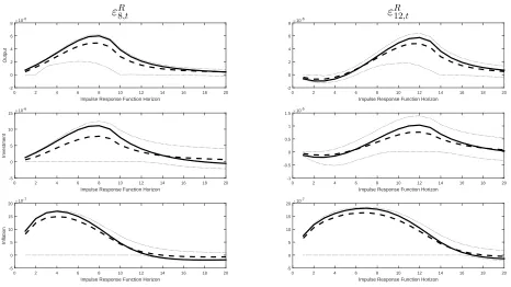
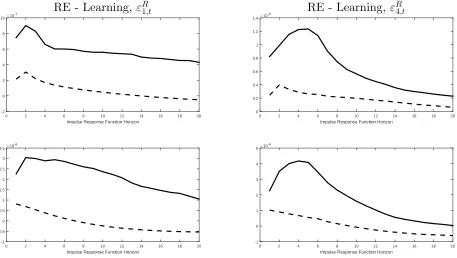
Figures 4 and 5 show that the addition of a financial sector into a standard New Keynesian

model amplifies the disparity between rational expectations and adaptive learning to forward

guid-ance. The top rows in the figures display the difference in output between the two expectations

formation schemes to forward guidance shocks under different values of ζspb. When the effect of

financial conditions on the economy diminishes, that is, ζspb = 0.001, the differences between

ra-tional expectations and adaptive learning to forward guidance reduce. However, when financial

factors are allowed to exist, that is, ζspb = 0.05, the disparity between the two increases. As

fi-nancial conditions play a bigger role in the economy, a bigger “wedge” exists between the output

responses of rational expectations and adaptive learning to forward guidance. Thus, the removal

of financial frictions from standard DSGE models leaves out an important channel through which

forward guidance operates.

The impulse responses of investment in the bottom rows of Figures 4 and 5 also show how

the addition of a financial sector can exacerbate the differences between rational expectations

and adaptive learning to forward guidance statements. The same type of large wedge that exists

between rational expectations and adaptive learning under output is apparent under investment.

When credit frictions play a larger role on the economy (e.g. ζspb= 0.05), adaptive learning agents’

forecasting model is more influenced by the financial sector. Thus, bigger differences between

rational expectations and adaptive learning exist.

This exacerbated difference can also be seen when examining the results of this paper in

comparison to a DSGE model in which the financial sector is removed. In Cole (2015), the model

of the economy was based on a smaller scale DSGE model without financial frictions. During an

economic crisis and in response to forward guidance, output was lower under adaptive learning than

rational expectations. With the inclusion of a financial sector in the present paper, the differences

in output between rational expectations and adaptive learning during the economic crisis exercise

in Section 4.3 are larger than in Cole (2015). The addition of the financial sector includes more

inertia in the PLM and more variables to forecast (e.g. EtR˜kt+1), and thus, more overall differences

between rational expectations and adaptive learning. The adaptive learning agents must estimate

how forward guidance will alleviate the recession by forecasting not only future variables concerning

households and firms, but also the financial sector. This creates more errors by the adaptive learning

to be greatly overstated under rational expectations relative to adaptive learning.

Overall, the findings in this section suggest a key takeaway for policymakers. If monetary

policymakers want to understand the effects of forward guidance and utilize macroeconomic models

with the standard assumptions of rational expectations and frictionless financial markets, the results

may be potentially misleading. This section shows that the addition of financial frictions into

a standard macroeconomic model exacerbates the differences between the responses of rational

expectations and adaptive learning to forward guidance.

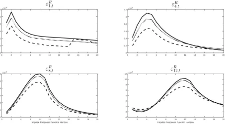
4.5 Alternative Constant Gains

This section examines the importance of financial frictions for forward guidance effectiveness when

the degree in which adaptive learning agents discount previous observations is changed.

Specifi-cally, the financial friction “wedge” that exists between the responses of rational expectations and

adaptive learning to forward guidance is examined to see how sensitive it is to different values of ¯τ.

The exercise in Section 4.2 is rerun under the baseline value ofζspb= 0.05. Lower and higher values

of ¯τ are also chosen. To capture adaptive learning agents placing less weight on new information,

the results are examined under ¯τ = 0.001 represented by the dotted line in Figure 6. To capture

adaptive learning agents placing more weight on new information, the results are examined under

¯

τ = 0.03 represented by the dashed line. The benchmark rational expectations impulse response

functions are also displayed and denoted by the solid line in Figure 6.

Figure 6 shows that the degree in which financial frictions amplify the differences between

rational expectations and adaptive learning depends on the value of ¯τ. When adaptive learning

agents place more weight on previous observations, that is, as ¯τ increases, financial conditions in

the economy have a bigger impact on their forecasts. Thus, output does not exhibit as strong of a

response to forward guidance as under a lower value of ¯τ. Figure 6 shows a larger wedge between

rational expectations and adaptive learning to forward guidance under ¯τ = 0.03 than ¯τ = 0.001

from the time of the announcement of the forward guidance shock to its realization. As adaptive

learning agents weight previous observations less, that is, as ¯τ decreases, their beliefs and forecasts

should not vary as much from the previous period. Consequently, current financial conditions in the

economy do not play as big of a role in their forecasts. Thus, the financial friction wedge between

rational expectations and adaptive learning diminishes. Figure 6 shows the smaller difference

between rational expectations and CGL with ¯τ = 0.001 from the time of the announcement of the

5

Conclusion

The 2007-2009 global financial crisis caused central banks around the world to implement the

unconventional monetary policy of forward guidance to stimulate their economies. The effectiveness

of forward guidance hinges on two key channels–expectations and financial markets–that are largely

overlooked in standard macroeconomic models. The standard expectations formation assumption

is the rational expectations hypothesis, while frictionless financial markets are largely assumed for

convenience. Thus, it is of interest to investigate the effectiveness of forward guidance when the

rational expectations assumption has been relaxed and credit frictions are included.

This paper utilizes a medium scale DSGE model with financial frictions to compare the effects

of forward guidance under both rational expectations and adaptive learning. The results show that

the addition of financial markets into a DSGE model amplifies the differences between rational

expectations and adaptive learning to forward guidance statements. Adaptive learning agents do

not respond as strongly to a forward guidance shock relative to their rational expectations

coun-terparts. During a period of economic crisis (e.g. a recession), output under rational expectations

also displays more favorable responses to forward guidance than under adaptive learning. Rational

expectations agents form their forecasts based on the true model of the economy, and thus, can

un-derstand how forward guidance will precisely help the economy. However, adaptive learning agents

must estimate the effects of forward guidance on the economy as their forecasts are based on an

econometric model of the economy. In addition, the differences between the responses of rational

expectations and adaptive learning to forward guidance reduce as the effect of financial frictions

in the model diminishes. These differences between the two expectations formations are also

mag-nified when compared to an analysis without financial frictions (e.g. Cole [2015]). The additional

inertia in the PLM, more financial sector variables to forecast, and the fact that adaptive learning

agents estimate the effects of forward guidance create bigger differences between the two types of

expectation assumptions. Furthermore, these results are especially important to policymakers. If

they want to understand the effects of forward guidance on the economy, monetary policymakers

should consider the way in which expectations and financial frictions are modeled.

There are other modifications to the model presented in this paper that are worth noting.

For example, the credibility of central bank forward guidance announcements could be examined

as in Dong (2014). In the model presented above, agents believe the forward guidance statements,

and the central bank implements its forward guidance promises. However, the results could be

examined when agents do not completely believe the central bank will follow through with its

paper examines time-contingent forward guidance in which the central bank communicates the end

date of forward guidance. Forward guidance could be state-contingent in which the completion

date of central bank forward guidance is linked to economic conditions (e.g. unemployment rate

and output). The RLS formula could also be modified to allow agents to better track structural

changes in the economy as described in Marcet and Nicolini (2003) and Milani (2014). Specifically,

the gain parameter would be a constant if the recent prediction errors were large and decreasing

if the recent prediction errors were small. Overall, the roles of expectations and financial frictions

References

Bernanke, B. S., Gertler, M., and Gilchrist, S. (1999). The financial accelerator in a quantitative

business cycle framework. Handbook of macroeconomics, 1:1341–1393.

Branch, W. A. and Evans, G. W. (2006). A simple recursive forecasting model.Economics Letters,

91(2):158–166.

Calvo, G. (1983). Staggered prices in a utility-maximizing framework. Journal of Monetary

Economics, 12(3):383–398.

Caputo, R., Medina, J. P., and Soto, C. (2010). The financial accelerator under learning and the

role of monetary policy. Documentos de Trabajo (Banco Central de Chile), (590):1.

Carlstrom, C., Fuerst, T., and Paustian, M. (2012). Inflation and output in new

keyne-sian models with a transient interest rate peg (Working Paper No. 459). Retrieved from: http://www.bankofengland.co.uk/research/documents/workingpapers/2012/wp459.pdf.

Christiano, L., Motto, R., and Rostagno, M. (2009). Financial factors in economic fluctuations.

Manuscript, Northwestern University and European Central Bank.

Cole, S. (2015). Learning and the effectiveness of central bank forward guidance. Technical report, Working paper, UC-Irvine.

De Graeve, F., Ilbas, P., and Wouters, R. (2014). Forward guidance and long term interest rates:

Inspecting the mechanism. Sveriges Riksbank Working Paper Series, (292).

Del Negro, M., Eusepi, S., Giannoni, M. P., Sbordone, A. M., Tambalotti, A., Cocci, M., Hasegawa,

R., and Linder, M. H. (2013). The frbny dsge model. FRB of New York Staff Report, (647).

Del Negro, M., Giannoni, M., and Patterson, C. (2012). The forward guidance puzzle. FRB of

New York Staff Report, (574).

Dong, B. (2014). Forward guidance and credible monetary policy. Technical report, Working paper, University of Virginia.

Eggertsson, G. B. and Woodford, M. (2003). The zero bound on interest rates and optimal

monetary policy. Brookings Papers on Economic Activity, (1):139–211.

Eusepi, S. and Preston, B. (2010). Central bank communication and expectations stabilization.

American Economic Journal: Macroeconomics, 2(3):235–271.

Eusepi, S. and Preston, B. (2011). Expectations, learning, and business cycle fluctuations.

Amer-ican Economic Review, 101(6):2844–72.

Evans, G. W. and Honkapohja, S. (2001).Learning and expectations in macroeconomics. Princeton

University Press.

Evans, G. W. and Honkapohja, S. (2013). Learning as a rational foundation for macroeconomics

and finance. Rethinking Expectations: The Way Forward for Macroeconomics, 68.

Evans, G. W., Honkapohja, S., and Mitra, K. (2009). Anticipated fiscal policy and adaptive

learning. Journal of Monetary Economics, 56(7):930–953.

Gilchrist, S., Ortiz, A., and Zakrajˇsek, E. (2009). Credit risk and the macroeconomy: Evidence

from an estimated dsge model. Unpublished manuscript, Boston University.

Honkapohja, S. and Mitra, K. (2005). Performance of inflation targeting based on constant interest

rate projections. Journal of Economic Dynamics and Control, 29(11):1867–1892.

Klenow, P. J. and Malin, B. A. (2010). Microeconomic evidence on price-setting. Handbook of

Monetary Economics, 3:231–284.

Kool, C. J. and Thornton, D. L. (2012). How effective is central bank forward guidance? FRB of

Kreps, D. M. (1998). Anticipated utility and dynamic choice. In Jacobs, D. P., Kalai, E., and

Kamien, M. I., editors,Frontiers of Research in Economic Theory: The Nancy L. Schwartz

Memo-rial Lectures, pages 242–274. Cambridge University Press.

Las´een, S. and Svensson, L. E. (2011). Anticipated alternative policy rate paths in policy

simula-tions. International Journal of Central Banking.

Levin, A., L´opez-Salido, D., Nelson, E., and Yun, T. (2010). Limitations on the effectiveness of

forward guidance at the zero lower bound. International Journal of Central Banking.

Marcet, A. and Nicolini, J. P. (2003). Recurrent hyperinflations and learning. The American

Economic Review, 93(5):1476–1498.

Marcet, A. and Sargent, T. J. (1989). Convergence of least squares learning mechanisms in

self-referential linear stochastic models. Journal of Economic Theory, 48(2):337–368.

McKay, A., Nakamura, E., and Steinsson, J. (2015). The power of forward guidance revisited. Technical report, National Bureau of Economic Research.

Milani, F. (2007). Expectations, learning and macroeconomic persistence. Journal of Monetary

Economics, 54(7):2065–2082.

Milani, F. (2014). Learning and time-varying macroeconomic volatility. Journal of Economic

Dynamics and Control, 47:94–114.

Mitra, K., Evans, G. W., and Honkapohja, S. (2012). Fiscal policy and learning. Bank of Finland

Research Discussion Paper, (5).

Orphanides, A. and Williams, J. C. (2005). The decline of activist stabilization policy: Natural

rate misperceptions, learning, and expectations. Journal of Economic Dynamics and Control,

29(11):1927–1950.

Schmitt-Groh´e, S. and Uribe, M. (2012). What’s news in business cycles. Econometrica,

80(6):2733–2764.

Sims, C. A. (2002). Solving linear rational expectations models. Computational Economics,

20(1):1–20.

Slobodyan, S. and Wouters, R. (2012). Learning in an estimated medium-scale dsge model.Journal

of Economic Dynamics and control, 36(1):26–46.

Smets, F. and Wouters, R. (2007). Shocks and frictions in us business cycles: A bayesian dsge

approach. The American Economic Review, 97(3):586–606.

Swanson, E. T. and Williams, J. C. (2014). Measuring the effect of the zero lower bound on

medium-and longer-term interest rates. American Economic Review, 104(10):3154–3185.

Woodford, M. (2003). Interest and prices: Foundations of a theory of monetary policy. princeton

university press.

Woodford, M. (2005). Central bank communication and policy effectiveness. In The Greenspan

Era: Lessons for the Future, pages 399–474. Federal Reserve Bank of St. Louis.

Woodford, M. (2010). Robustly optimal monetary policy with near-rational expectations. The

American Economic Review, pages 274–303.

Woodford, M. (2012). Methods of policy accommodation at the interest-rate lower bound. In