A regression model of product differentiation

Munich Personal RePEc Archive

A regression model of product

differentiation

Mogens, Fosgerau

Danish Technical University

1 July 2016

Online at

https://mpra.ub.uni-muenchen.de/72786/

A regression model of product differentiation

Mogens Fosgerau

July 29, 2016

Abstract

This paper develops a model of product differentiation that can be estimated using stan-dard regression techniques and applies it to a panel data set of new car sales. The model allows for complex substitution patterns according to an overlapping nest structure that makes cars closer substitutes if the share brand, body type, and/or quality level. A nest comprising all the car alternatives ensure that they are closer substitutes with each other than with the outside good. In addition, the model comprises fixed effects by car model, controlling for unobserved car quality.

1

Introduction

This note provides a model to estimate the demand for a differentiated product that allows for complex substitution patterns and numerous fixed effects. The models is estimated using standard regression techniques without any convergence issues. The model is a specific instance of the generalized entropy model proposed byFosgerau and de Palma(2016). It is here applied to a publicly available market level panel data set of new car sales covering 250 different kinds of cars, 5 countries and 30 years.

Modeling new car sales entails two fundamental issues that arise in many similar situations. The first issue is that the quality of cars is correlated with price but imperfectly observed; this creates an endogeneity issue. The second issue is the presence of complex substitution patterns that are not well described by a simple model such as the logit model.

stability of BLP and finds that results can be critically unstable, even when the procedure is well carried out.

It is then desirable to have a way to deal with endogeneity and complex substitution patterns that does not suffer from the drawbacks of the BLP model. This note presents such a model that is applicable to panel data of market shares.

Generalized entropy models were proposed byFosgerau and de Palma(2016) (FdP, hence-forth). It is a general class of models that comprises dual representations of all ARUM as well as more general models. This note applies a particular instance of generalized entropy models that generalizes the nested logit model by allowing arbitrarily overlapping nests.

2

Model formulation

A representative consumer with income y faces goods j = 0; :::J, where j = 1; :::; J are different car models and0is an outside good. Demand for cars isq = (q0; q1; :::; qJ), which is

non-negative and sums to 1, i.e.,q 2 , where is the unit simplex. Each car has an associated price pj and qualityvj, while p0 = v0 = 0. Income is sufficiently large thaty > maxjfpjg.

The representative consumer chooses demand to maximize utility

u(q) = y+q (v p) + (q);

where > 0is a constant marginal utility of income and is a generalized entropy with the following properties (from FdP): it is a concave function : [0;1)J+1 !R[ f 1ggiven by

(q) = q lnS(q); q2

1; q =2 ; (2.1)

whereS: [0;1)J+1 ! [0;1)J+1 is continuous, homogenous of degree 1, and globally invert-ible. Furthermore,Sis differentiable at anyq2relint ( )with

J X

j=1

qj

@lnS(j)_(q)

@qk

= ; k 2 f1; :::; Jg;

where >0.

Utility maximization leads to demand

q(v; p) = H

(1)_(ev p₎ PJ

j=1H(j)(ev p)

; :::; H

(J)_(ev p₎ PJ

j=1H(j)(ev p) !

whereH =S 1 _{is the inverse ofS. Moreover,}

lnS(q) = (v p) +c; (2.3)

wherec2_Ris a constant that depends on(v p).

As shown by FdP, this class of models comprises dual representations of all ARUM discrete choice models. For example, when S(q) = q is the identity, then also H is the identity and demand is just logit demand.

Another illustrative example is the nested logit model. Partition the set of alternatives

f0;1; :::; Jg into nestsg 2 G, denote by gj the nest that contains alternative j, and let qg = P

j2gqj. Then define

S(j)(q) = q_jgjqg1j gj; j = 0; :::J (2.4)

where _g 2]0;1]are parameters. ThenSsatisfies the conditions given. With this specification ofS, the generalized entropy contains termsqj 1 gj lnqgj that makes alternatives in the

same nests closer substitutes (perfect substitutes if _gj = 1). The resulting demand is

qj =

e

vj pj gj

P i2gje

vi pi gj

e gj

ln

0

@P_i2_gje

vi pi gj

1

A

P g2Ge

gln

P

i2ge vi pi

g

!;

which is the nested logit model.

Here we shall employ a more general version of this that allows for overlapping nests. The set of alternativesf0;1; :::; Jgis grouped according to different criteriac. A criterioncassigns a value to each element of f0; :::; Jg. Alternatives are grouped together on criterioncif they are assigned the same value byc. Then defining c(j) = fkjc(k) =c(j)g, c(j)is the set of

alternatives grouped with alternative J on criterion c. Define nesting parameters _c > 0with

P

c c <1and let 0 = 1 P

c c. Then define for allj

S(j)_{(q) = q} 0

j Q

c

q c c(j):

As shown in FdP, this satisfies the conditions set out above. As before, each termq c

c(j) makes

alternatives closer substitutes if they belong to the same nest on criterionc, where the degree of substitutability is controlled by the parameter _c.

From (2.3) we obtain that

0lnqj + P

c c

Since ₀ >0we may equivalently write

lnqj =

P c

c 0

lnq c(j)+

1

0

vj 0

pj +

c

0

; (2.5)

which suggests that this model may be estimated using regression.

3

Empirical model formulation

We employ panel data giving new car sales in countries indexed by m, and years indexed by

t. Alternative j = 0 is the outside alternative. A nesting structure is defined for the inside alternatives. Equation (2.5) is then be elaborated into

lnqjmt =

P c c

lnq c(j);mt+ xjmt+ j + mt+ jmt; j >0 (3.1a)

lnq0mt = 0+ mt+ 0mt; (3.1b)

where the structural parameters _c may be recovered from _c = _c= ₀ using ₀ = 1

1+P_c c

,

c = c 0, since 0+

P

c c = 1.

Going through the terms in (3.1) one by one, this means that the log market share for carj

depends first on the log market share for cars that belong to the same category as carj on each of the criteriac. Second, the qualitiesvj are parametrized by xjmt+ j. Explanatory variables

inxjmtinclude observable car characteristics that change across countries and years as well as

price. All other aspects of car quality are captured by the fixed effect _j. Third, country and year specific fixed effects _mtallow the constantcin (2.5) to be omitted. Finally, random shocks

jmtare included and assumed to be mean independent of(x; ).

The model has thus been translated into a regression model with panel data. One issue re-mains, namely that termslnq c(j);mt are endogenous, since they depend on the random shocks

jmt. There are instruments available within the model, that are constructed by averaging

inde-pendent variables across nests:

x c(j);mt =

1

j c(j)j P i2 c(j)

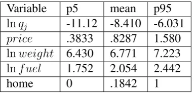
Variable p5 mean p95

lnqj -11.12 -8.410 -6.031

price .3833 .8287 1.580 lnweight 6.430 6.771 7.223 lnf uel 1.752 2.054 2.442

home 0 .1842 1

Table 1: Summary statistics

4

Data and estimation results

The data are from Frank Verboven’s website (https://sites.google.com/site/frankverbo/), down-loaded June 2014. The dataset covers five countries (Belgium, France, Germany, Italy, and the UK) over the 30 year period 1970-1999. Car models are grouped into 262 representative cars that cover most of sales during the period. The share for the outside good is taken to be the size of the population minus the total car sales in each country and year. The data comprises 11447

observations of annual car sales by country, year and car. Table 1 provides some summary

statistics.

The models presented below use the following categorizations of car alternatives to form nests: The first categorization variable distinguishes inside goods from the outside good, such that all inside goods can be closer substitutes with each other than with the outside good. The second categorization used is the car class, which divides cars into subcompact, compact, in-termediate, standard, and luxury. The third categorization is defined according to a perceived quality of different car brands.1 _{There are four quality categories: one for high quality cars,} pri-marily German and Swedish; one intermediate and one low quality category. A fourth category distinguishes the smaller Asian brands from the rest. The fourth categorization distinguishes between car producing firms.

The explanatory variables included inxare price, log weight, log fuel consumption, and a dummy for whether a car is produced domestically. The price variable is price relative to per capita GDP. To avoid overidentification, only the price variable is used to form instruments.

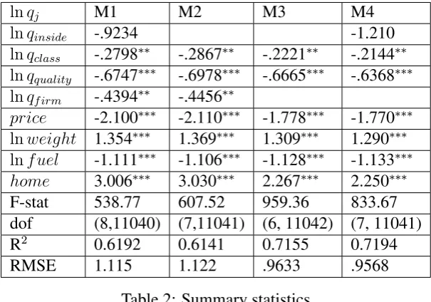
Models are estimated using the Stata module reghdfe (Correia, 2014), which allows for multiway fixed effects. This takes essentially zero time. Estimation results are provided in Table 2, which shows four models. The first, M1, includes four layers of nesting, as well as car price, weight, fuel consumption and a dummy indicating whether the car is produced domestically. All parameter estimates have the expected sign, but the nesting parameter for the inside alternatives lnqinsideis not significantly different from zero. Model M2 omitslnqinside;

this has only small effect on the other parameter estimates. Model M3 also omitslnqf irm, and

this leads to some change in the other parameter estimates. Model M4 adds backlnqinsidewith

lnqj M1 M2 M3 M4

lnqinside -.9234 -1.210

lnqclass -.2798 -.2867 -.2221 -.2144

lnqquality -.6747 -.6978 -.6665 -.6368

lnqf irm -.4394 -.4456

price -2.100 -2.110 -1.778 -1.770 lnweight 1.354 1.369 1.309 1.290 lnf uel -1.111 -1.106 -1.128 -1.133

home 3.006 3.030 2.267 2.250

F-stat 538.77 607.52 959.36 833.67

dof (8,11040) (7,11041) (6, 11042) (7, 11041)

R2 0.6192 0.6141 0.7155 0.7194

RMSE 1.115 1.122 .9633 .9568

Table 2: Summary statistics

Parameter significance indicated using *:p<_10%,**:p<_1%,***:p<_0.1%

are not much affected. All models pass tests for underidentification.

5

Generating counterfactuals

This section illustrates how the generalized entropy model may be used to create counterfactual scenarios. Let q0 _{be these market shares and use (3.1) to compute v}0 _{= lnS(q}1_{). Say a}

counterfactual scenario changes x0 _{to x}1 _{and define v}1 _{= v}0 _{+ (x}1 _x0_{). Then, from}

(2.3), counterfactual demandq1 _{may be found by solving}

lnS q1 =v1+c; (5.1)

wherecis a normalizing constant ensuring that demand sums to 1. FdP shows that this equation has a unique solution and that the following iteration always converges to this solution. Given a current candidate solutionq(n)_{, the next candidate is found as}

q(n+1)j =

qj(n)e v1

j=S(j) q(n)

P k

q_k(n)ev1

k=S(k)(q(n))

; (5.2)

and the iteration stops when the change from q(n) _{to q}(n+1) _{is small. The intuition for (5.2)}

is straightforward: The numerator adjusts qj(n) in the direction required by (5.1), while the

denominator ensures that demand sums to 1.

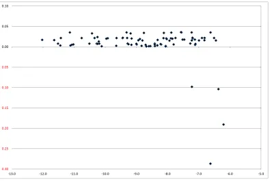
the outside good. The example uses the market shares for the UK in the year 1999. The iteration (5.2) was implemented in a spreadsheet.

The price of Ford cars was raised by 20% in the counterfactual scenario. This kind of change allows the substitution patterns to be understood quite intuitively. Overall, the model is able to describe a rich pattern of cross-elasticities as shown in Figure1, which shows a scatter plot of the change in demand,lnq1 _lnq0_{, against the base demandlnq}0_.

0.30 0.25 0.20 0.15 0.10 0.05

0.00 0.05 0.10

‐13.0 ‐12.0 ‐11.0 ‐10.0 ‐9.0 ‐8.0 ‐7.0 ‐6.0 ‐5.0

Figure 1: The change in log demand (vertical axis) against observed log demand (horizontal axis) for the 85 car models present on the UK market in 19999

References

Aguirregabiria, V. and Mira, P. (2010) Dynamic discrete choice structural models: A survey

Journal of Econometrics156(1), 38–67.

Berry, S., Levinsohn, J. and Pakes, A. (1995) Automobile Prices in Market Equilibrium Econo-metrica63(4), 841–890.

Correia, S. (2014)REGHDFE: Stata module to perform linear or instrumental-variable regres-sion absorbing any number of high-dimenregres-sional fixed effects. Published: Statistical Software Components, Boston College Department of Economics.

Fosgerau, M. and de Palma, A. (2016) Generalized entropy models.

Fosgerau, M., Frejinger, E. and Karlstrom, A. (2013) A link based network route choice model with unrestricted choice setTransportation Research Part B: Methodological56, 70–80.

Knittel, C. R. and Metaxoglou, K. (2014) Estimation of Random-Coefficient Demand Models: Two Empiricists’ PerspectiveReview of Economics and Statistics96(1), 34–59.