Factoring Synchronous Grammars by Sorting

Factoring Synchronous Grammars By Sorting

Daniel Gildea Computer Science Dept.

University of Rochester Rochester, NY 14627

Giorgio Satta Dept. of Information Eng’g

University of Padua I-35131 Padua, Italy

Hao Zhang Computer Science Dept.

University of Rochester Rochester, NY 14627

Abstract

Synchronous Context-Free Grammars (SCFGs) have been successfully exploited as translation models in machine trans-lation applications. When parsing with an SCFG, computational complexity grows exponentially with the length of the rules, in the worst case. In this paper we examine the problem of factorizing each rule of an input SCFG to a generatively equivalent set of rules, each having the smallest possible length. Our algorithm works in time O(nlogn), for each rule

of lengthn. This improves upon previous

results and solves an open problem about recognizing permutations that can be factored.

1 Introduction

Synchronous Context-Free Grammars (SCFGs) are a generalization of the Context-Free Gram-mar (CFG) formalism to simultaneously produce strings in two languages. SCFGs have a wide range of applications, including machine transla-tion, word and phrase alignments, and automatic dictionary construction. Variations of SCFGs go back to Aho and Ullman (1972)’s Syntax-Directed Translation Schemata, but also include the In-version Transduction Grammars in Wu (1997), which restrict grammar rules to be binary, the syn-chronous grammars in Chiang (2005), which use only a single nonterminal symbol, and the Multi-text Grammars in Melamed (2003), which allow independent rewriting, as well as other tree-based models such as Yamada and Knight (2001) and Galley et al. (2004).

When viewed as a rewriting system, an SCFG generates a set of string pairs, representing some translation relation. We are concerned here with the time complexity of parsing such a pair, accord-ing to the grammar. Assume then a pair with each

string having a maximum length of N, and

con-sider an SCFG Gof size |G|, with a bound ofn

nonterminals in the right-hand side of each rule in a single dimension, which we call below therank

ofG. As an upper bound, parsing can be carried

out in timeO(|G|Nn+4)by a dynamic

program-ming algorithm maintaining continuous spans in one dimension. As a lower bound, parsing strate-gies with discontinuous spans in both dimensions can take timeΩ(|G|Nc√n)for unfriendly

permu-tations (Satta and Peserico, 2005). A natural ques-tion to ask then is: What if we could reduce the rank of G, preserving the generated translation?

As in the case of CFGs, one way of doing this would be to factorize each single rule into several rules of rank strictly smaller thann. It is not

diffi-cult to see that this would result in a new grammar of size at most 2· |G|. In the time complexities reported above, we see that such a size increase would be more than compensated by the reduction in the degree of the polynomial in N. We thus

conclude that a reduction in the rank of an SCFG would result in more efficient parsing algorithms, for most common parsing strategies.

In the general case, normal forms with bounded rank are not admitted by SCFGs, as shown in (Aho and Ullman, 1972). Nonetheless, an SCFG with a rank ofnmay not necessarily meet the worst case

of Aho and Ullman (1972). It is then reasonable to ask if our SCFGGcan be factorized, and what

is the smallest rank k < n that can be obtained

in this way. This paper answers these two ques-tions, by providing an algorithm that factorizes the rules of an input SCFG, resulting in a new, genera-tively equivalent, SCFG with rankkas low as

pos-sible. The algorithm works in timeO(nlogn)for

each rule, regardless of the rankkof the factorized

rules. As discussed above, in this way we achieve an improvement of the parsing time for SCFGs, obtaining an upper bound ofO(|G|Nk+4)by

us-ing a parsus-ing strategy that maintains continuous

1,2

1,2

2,1

2 1 1,2

3 4

3,1,4,2

7 5 8 6

4,1,3,5,2

7 1 2,4,1,3

4 6 3 5 8 2

Figure 1: Two permutation trees. The permuta-tions associated with the leaves can be produced by composing the permutations at the internal nodes.

spans in one dimension.

Previous work on this problem has been pre-sented in Zhang et al. (2006), where a method is provided for casting an SCFG to a form with rank

k= 2. If generalized to any value ofk, that

algo-rithm would run in timeO(n2). We thus improve

existing factorization methods by almost a factor ofn. We also solve an open problem mentioned

by Albert et al. (2003), who pose the question of whether irreducible, or simple, permutations can be recognized in time less thanΘ(n2).

2 Synchronous CFGs and permutation trees

We begin by describing the synchronous CFG for-malism, which is more rigorously defined by Aho and Ullman (1972) and Satta and Peserico (2005). Let us consider strings defined over some set of nonterminal and terminal symbols, as defined for CFGs. We say that two such strings are syn-chronous if some bijective relation is given

be-tween the occurrences of the nonterminals in the two strings. Asynchronous context-free gram-mar (SCFG) is defined as a CFG, with the

dif-ference that it uses synchronous rules of the form

[A1 → α1, A2 →α2], withA1, A2nonterminals

andα1, α2 synchronous strings. We can use

pro-duction[A1 →α1, A2 →α2]to rewrite any

syn-chronous strings [γ11A1γ12, γ21A2γ22] into the

synchronous strings [γ11α1γ12, γ21α2γ22],

un-der the condition that the indicated occurrences of A1 and A2 be related by the bijection

asso-ciated with the source synchronous strings. Fur-thermore, the bijective relation associated with the target synchronous strings is obtained by compos-ing the relation associated with the source syn-chronous strings and the relation associated with synchronous pair [α1, α2], in the most obvious

way.

As in standard constructions that reduce the

rank of a CFG, in this paper we focus on each single synchronous rule and factorize it into syn-chronous rules of lower rank. If we view the bijec-tive relation associated with a synchronous rule as a permutation, we can further reduce our factoriza-tion problem to the problem of factorizing a per-mutation of arityninto the composition of several

permutations of arity k < n. Such factorization

can be represented as a tree of composed permuta-tions, called in what follows apermutation tree.

A permutation tree can be converted into a set of

k-ary SCFG rules equivalent to the input rule. For

example, the input rule:

[X→A(1)B(2)C(3)D(4)E(5)F(6)G(7)H(8), X→B(2)A(1)C(3)D(4)G(7)E(5)H(8)F(6)]

yields the permutation tree of Figure 1(left). In-troducing a new grammar nonterminalXifor each

internal node of the tree yields an equivalent set of smaller rules:

[X →X₁(1)X₂(2), X →X₁(1)X₂(2)]

[X1→X3(1)X (2)

4 , X1 →X3(1)X (2) 4 ] [X₃→A(1)B(2), X₃ →B(2)A(1)] [X4→C(1)D(2), X4 →C(1)D(2)] [X2→E(1)F(2)G(3)H(4),

X2→G(3)E(1)H(4)F(2)]

In the case of stochastic grammars, the rule cor-responding to the root of the permutation tree is assigned the original rule’s probability, while all other rules, associated with new grammar nonter-minals, are assigned probability 1. We process each rule of an input SCFG independently, pro-ducing an equivalent grammar with the smallest possible arity.

3 Factorization Algorithm

In this section we specify and discuss our factor-ization algorithm. The algorithm takes as input a permutation defined on the set{1,· · · , n}, repre-senting a rule of some SCFG, and provides a per-mutation tree of arityk≤nfor that permutation,

withkas small as possible.

tree, it is safe to greedily reduce a subsequence into a new subtree as soon as a subsequence is found which represents a continuous span in both dimensions of the permutation matrix1_associated with the input permutation. For space reasons, we omit the proof, but emphasize that any greedy re-duction turns out to be either necessary, or equiv-alent to the other alternatives.

Any sequences of binary rules can be rear-ranged into a normalized form (e.g. always left-branching) as a postprocessing step, if desired.

The top-level structure of the algorithm exploits a divide-and-conquer approach, and is the same as that of the well-known mergesort algorithm (Cor-men et al., 1990). We work on subsequences of the original permutation, and ‘merge’ neighbor-ing subsequences into successively longer subse-quences, combining two subsequences of length

2iinto a subsequence of length

2i₊₁until we have

built one subsequence spanning the entire permu-tation. If each combination of subsequences can be performed in linear time, then the entire permu-tation can be processed in timeO(nlogn). As in

the case of mergesort, this is an application of the so-called master theorem (Cormen et al., 1990).

As the algorithm operates, we will maintain the invariant that we must have built all subtrees of the target permutation tree that are entirely within a given subsequence that has been processed. This is analogous to the invariant in mergesort that all processed subsequences are in sorted order. When we combine two subsequences, we need only build nodes in the tree that cover parts of both sub-sequences, but are entirely within the combined subsequence. Thus, we are looking for subtrees that span the midpoint of the combined subse-quence, but have left and right boundaries within the boundaries of the combined subsequence. In what follows, this midpoint is called the split point.

From this invariant, we will be guaranteed to have a complete, correct permutation tree at the end of last subsequence combination. An example of the operation of the general algorithm is shown in Figure 2. The top-level structure of the algo-rithm is presented in function KARIZEof Figure 3.

There may be more than one reduction neces-sary spanning a given split point when combin-ing two subsequences. Function MERGE in

Fig-1_{A permutation matrix is a way of representing a}

permuta-tion, and is obtained by rearranging the row (or the columns) of an identity matrix, according to the permutation itself.

2 1 3 4 7 5 8 6

2,1

2 1

1,2

3 4 7 5 8 6

1,2

2,1

2 1 1,2

3 4

3,1,4,2

7 5 8 6

1,2

1,2

2,1

2 1 1,2

3 4

3,1,4,2

7 5 8 6

Figure 2: Recursive combination of permutation trees. Top row, the input permutation. Second row, after combination into sequences of length two, bi-nary nodes have been built where possible. Third row, after combination into sequences of length four; bottom row, the entire output tree.

ure 3 initializes certain data structures described below, and then checks for reductions repeatedly until no further reduction is possible. It looks first for the smallest reduction crossing the split point of the subsequences being combined. If SCAN,

described below, finds a valid reduction, it is com-mitted by calling REDUCE. If a reduction is found,

we look for further reductions crossing either the left or right boundary of the new reduction, repeat-ing until no further reductions are possible. Be-cause we only need to find reductions spanning the original split point at a given combination step, this process is guaranteed to find all reductions needed.

We now turn to the problem of identifying a specific reduction to be made across a split point, which involves identifying the reduction’s left and right boundaries. Given a subsequence and can-didate left and right boundaries for that subse-quence, the validity of making a reduction over this span can be tested by verifying whether the span constitutes a permuted sequence, that is,

condi-functionKARIZE(π)

. initialize with identity mapping

h←hmin←hmax←(0..|π|);

. mergesort core for size←1;size≤ |π|;size←size* 2do

for min←0;

min<|π|-size+1; min←min+ 2 *size do div=min+size- 1;

max←min(|π|,min+ 2*size- 1); MERGE(min,div,max);

functionMERGE(min,div,max)

. initializeh sorth[min..max] according toπ[i];

sorthmin[min..max] according toπ[i];

sorthmax[min..max] according toπ[i]; . merging sorted list takes linear time

. initializev

for i←min;i≤max;i←i+ 1 do

v[h[i] ]←i;

. check if start of new reduced block if i=minor

hmin[i]6=hmin[i-1] then

vmin←i; vmin[h[i] ]←vmin;

for i←max;i≥min;i←i- 1do

. check if start of new reduced block if i=maxor

hmax[i]6=hmax[i+1] then

vmax←i; vmax[h[i] ]←vmax;

. look for reductions ifSCAN(div) then

REDUCE(scanned reduction);

while SCAN(left) or SCAN(right) do

REDUCE(smaller reduction);

functionREDUCE(left,right,bot,top)

for i←bot..top do hmin[i]←left; hmax[i]←right;

for i←left..right do vmin[i]←bot; vmax[i]←top; print “reduce:”left..right;

Figure 3: KARIZE: Top level of algorithm,

iden-tical to that of mergesort. MERGE: combines two

subsequences of size2i into new subsequence of

size2i₊₁. R_EDUCE: commits reduction by

updat-ingminandmaxarrays.

tion can be tested by scanning the span in ques-tion, finding the minimum and maximum integers in the span, and checking whether their difference is equal to the length of the span minus one. Be-low we call this condition thereduction test. As

an example of the reduction test, consider the sub-sequence (7,5,8,6), and take the last three

ele-ments, (5,8,6), as a candidate span. We see that 5 and8 are the minimum and maximum integers

in the corresponding span, respectively. We then compute8−5 = 3, while the length of the span

minus one is2, implying that no reduction is

possi-ble. However, examining the entire subsequence, the minimum is 5 and the maximum is 8, and 8−5 = 3, which is the length of the span minus

one. We therefore conclude that we can reduce that span by means of some permutation, that is, parse the span by means of a node in the permuta-tion tree. This reducpermuta-tion constitutes the 4-ary node in the permutation tree of Figure 2.

A trivial implementation of the reduction test would be to tests all combinations of left and right boundaries for the new reduction. Unfortunately, this would take time Ω(n2) for a single

subse-quence combination step, whereas to achieve the overallO(nlogn)complexity we need linear time

for each combination step.

It turns out that the boundaries of the next re-duction, covering a given split point, can be com-puted in linear time with the technique shown in function SCANof Figure 5. We start with left and

right candidate boundaries at the two points imme-diately to the left and right of the split point, and then repeatedly check whether the current left and right boundaries identify a permuted sequence by applying the reduction test, and move the left and right boundaries outward as necessary, as soon as ‘missing’ integers are identified outside the cur-rent boundaries, as explained below. We will show that, as we move outward, the number of possible configurations achieved for the positions of the left and the right boundaries is linearly bounded in the length of the combined subsequence (as opposed to quadratically bounded).

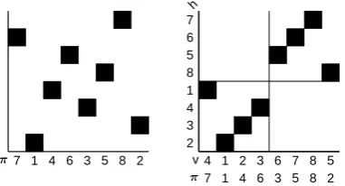
7 1 4 6 3 5 8 2

π ₄

7 2

1 1 3

2 4 4

3 6 1

6 3 8

7 5 5

8 8 6

5 2 7

v

π

h

Figure 4: Permutation matrix for input permuta-tion π (left) and within-subsequence permutation

v(right) for subsequences of size four.

maintain two arrays:h, which maps from vertical to horizontal positions within the current subse-quence, andvwhich maps from horizontal to ver-tical positions. These arrays represent the within-subsequence permutation obtained by sorting the elements of each subsequence according to the input permutation, while keeping each element within its block, as shown in Figure 4.

Within each subsequence, we alternate between scanning horizontally from left to right, possibly extending the top and bottom boundaries (Figure 5 lines 9 to 14), and scanning vertically from bottom to top, possibly extending the left and right bound-aries (lines 20 to 26). Each extension is forced when, looking at the within-subsequence permuta-tion, we find that some element is within the cur-rent boundaries in one dimension but outside the boundaries in the other. If the distance between vertical boundaries is larger in the input permu-tation than in the subsequence permupermu-tation, nec-essary elements are missing from the current sub-sequence and no reduction is possible at this step (line 18). When all necessary elements are present in the current subsequence and no further exten-sions are necessary to the boundaries (line 30), we have satisfied the reduction test on the input per-mutation, and make a reduction.

The trick used to keep the iterative scanning lin-ear is that weskipthe subsequence scanned on the previous iteration on each scan, in both the hori-zontal and vertical directions. Lines 13 and 25 of Figure 5 perform this skip by advancing thexandy counters past previously scanned regions. Consid-ering the horizontal scan of lines 9 to 14, in a given iteration of the while loop, we scan only the items between newleft and left and between right and newright. On the next iteration of the while loop, thenewleftboundary has moved further to the left,

1: function SCAN(div)

2: left← −∞; 3: right← −∞; 4: newleft←div; 5: newright←div+ 1 ;

6: newtop← −∞;

7: newbot← ∞;

8: while 1 do

. horizontal scan

9: for x←newleft;x≤newright; do

10: newtop←max(newtop,vmax[x]);

11: newbot←min(newbot,vmin[x]);

. skip to end of reduced block

12: x←hmax[vmin[x]] + 1;

. skip section scanned on last iter

13: if x=left then

14: x←right+ 1;

15: right←newright;

16: left←newleft;

. the reduction test

17: if newtop-newbot<

18: π[h[newtop]] -π[h[newbot]] then

19: return(0);

. vertical scan

20: for y←newbot;y≤newtop; do

21: newright←

22: max(newright,hmax[y]);

23: newleft←min(newleft,hmin[y]);

. skip to end of reduced block

24: y←vmax[hmin[y]] + 1;

. skip section scanned on last iter

25: if y=bot then

26: y←top+ 1;

27: top←newtop;

28: bot←newbot;

. if no change to boundaries, reduce

29: if newright=right

30: andnewleft=left then

31: return(1,left,right,bot,top);

while the variable lefttakes the previous value of newleft, ensuring that the items scanned on this it-eration are distinct from those already processed. Similarly, on the right edge we scan new items, between right and newright. The same analysis applies to the vertical scan. Because each item in the permutation is scanned only once in the verti-cal direction and once in the horizontal direction, the entire call to SCAN takes linear time,

regard-less of the number of iterations of the while loop that are required.

We must further show that each call to MERGE

takes only linear time, despite that fact that it may involve many calls to SCAN. We

accom-plish this by introducing a second type of skipping in the scans, which advances past any previously reduced block in a single step. In order to skip past previous reductions, we maintain (in func-tion REDUCE) auxiliary arrays with the minimum

and maximum positions of the largest block each point has been reduced to, in both the horizontal and vertical dimensions. We use these data struc-tures (hmin,hmax,vmin,vmax) when advancing to the next position of the scan in lines 12 and 24 of Figure 5. Because each call to SCANskips items

scanned by previous calls, each item is scanned at most twice across an entire call to MERGE,

once when scanning across a new reduction’s left boundary and once when scanning across the right boundary, guaranteeing that MERGEcompletes in

linear time.

4 An Example

In this section we examine the operation of the algorithm on a permutation of length eight, re-sulting in the permutation tree of Figure 1(right). We will build up our analysis of the permutation by starting with individual items of the input per-mutation and building up subsequences of length 2, 4, and finally 8. In our example permutation,

(7,1,4,6,3,5,8,2), no reductions can be made

until the final combination step, in which one per-mutation of size 4 is used, and one of size 5.

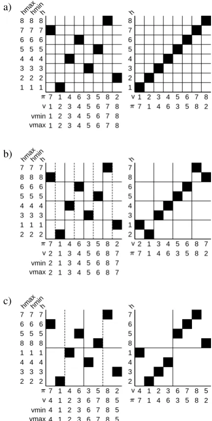
We begin with the input permutation along the bottom of Figure 6a. We represent the interme-diate data structures h,hmin, andhmaxalong the vertical axis of the figure; these three arrays are all initialized to be the sequence(1,2,· · · ,8).

Figure 6b shows the combination of individual items into subsequences of length two. Each new subsequence of the harray is sorted according to

a) 7 1 1 1 1 1 1 1 2 2 2 2 2 2 4 3 3 3 3 3 3 6 4 4 4 4 4 4 3 5 5 5 5 5 5 5 6 6 6 6 6 6 8 7 7 7 7 7 7 2 8 8 8 8 8 8 π v vmin vmax h hmin hmax 1 7 1 2 1 2 3 4 3 4 6 4 5 3 5 6 5 6 7 8 7 8 2 8 v π h b) 7 2 2 2 2 2 2 1 1 1 1 1 1 1 4 3 3 3 3 3 3 6 4 4 4 4 4 4 3 5 5 5 5 5 5 5 6 6 6 6 6 6 8 8 8 8 8 8 8 2 7 7 7 7 7 7 π v vmin vmax h hmin hmax 2 7 2 1 1 1 3 4 3 4 6 4 5 3 5 6 5 6 8 8 8 7 2 7 v π h c) 7 4 4 4 2 2 2 1 1 1 1 3 3 3 4 2 2 2 4 4 4 6 3 3 3 1 1 1 3 6 6 6 8 8 8 5 7 7 7 5 5 5 8 8 8 8 6 6 6 2 5 5 5 7 7 7 π v vmin vmax h hmin hmax 4 7 2 1 1 3 2 4 4 3 6 1 6 3 8 7 5 5 8 8 6 5 2 7 v π h

Figure 6: Steps in an example computation, with input permutation π on left and

a) 7 7 7 7 2 2 2 1 1 1 1 8 8 8 4 4 4 4 5 5 5 6 6 6 6 3 3 3 3 3 3 3 6 6 6 5 5 5 5 4 4 4 8 8 8 8 1 1 1 2 2 2 2 7 7 7 π v vmin vmax h hmin hmax b) 7 7 7 7 2 2 2 1 1 1 1 8 8 8 4 4 3 6 5 3 6 6 6 3 6 3 3 6 3 3 3 6 6 3 6 5 5 3 6 4 3 6 8 8 8 8 1 1 1 2 2 2 2 7 7 7 π v vmin vmax h hmin hmax

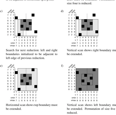
Left and right boundaries are initialized

to be adjacent to horizontal split point. Vertical scan shows left and right bound-aries must be extended. Permutation of size four is reduced.

c) 7 7 7 7 2 2 2 1 1 1 1 8 8 8 4 4 3 6 5 3 6 6 6 3 6 3 3 6 3 3 3 6 6 3 6 5 5 3 6 4 3 6 8 8 8 8 1 1 1 2 2 2 2 7 7 7 π v vmin vmax h hmin hmax d) 7 7 7 7 2 2 2 1 1 1 1 8 8 8 4 4 3 6 5 3 6 6 6 3 6 3 3 6 3 3 3 6 6 3 6 5 5 3 6 4 3 6 8 8 8 8 1 1 1 2 2 2 2 7 7 7 π v vmin vmax h hmin hmax

Search for next reduction: left and right boundaries initialized to be adjacent to left edge of previous reduction.

Vertical scan shows right boundary must be extended. e) 7 7 7 7 2 2 2 1 1 1 1 8 8 8 4 4 3 6 5 3 6 6 6 3 6 3 3 6 3 3 3 6 6 3 6 5 5 3 6 4 3 6 8 8 8 8 1 1 1 2 2 2 2 7 7 7 π v vmin vmax h hmin hmax f) 7 7 1 8 2 1 8 1 1 1 8 8 1 8 4 4 1 8 5 1 8 6 6 1 8 3 1 8 3 3 1 8 6 1 8 5 5 1 8 4 1 8 8 8 1 8 1 1 8 2 2 1 8 7 1 8 π v vmin vmax h hmin hmax

Horizontal scan shows top boundary must

be extended. Vertical scan shows left boundary mustbe extended. Permutation of size five is reduced.

Figure 7: Steps in scanning for final combination of subsequences, wherev = π. Area within current

the vertical position of the dots in the correspond-ing columns. Thus, becauseπ[7] = 8 > π[8] = 2,

we swap 7 and 8 in the h array. The algorithm checks whether any reductions can be made at this step by computing the difference between the in-tegers on each side of each split point. Because none of the pairs of integers in are consecutive, no reductions are made at this step.

Figure 6c shows the combination the pairs into subsequences of length four. The two split points to be examined are between the second and third position, and the sixth and seventh position. Again, no reductions are possible.

Finally we combine the two subsequences of length four to complete the analysis of the entire permutation. The split point is between the fourth and fifth positions of the input permutation, and in the first horizontal scan of these two positions, we see thatπ[4] = 6andπ[5] = 3, meaning our

top boundary will be 6 and our bottom boundary 3, shown in Figure 7a. Scanning vertically from position 3 to 6, we see horizontal positions 5, 3, 6, and 4, giving the minimum, 3, as the new left boundary and the maximum, 6, as the new right boundary, shown in Figure 7b. We now perform another horizontal scan starting at position 3, but then jumping directly to position 6, as horizontal positions 4 and 5 were scanned previously. Af-ter this scan, the minimum vertical position seen remains 3, and the maximum vertical position is still 6. At this point, because we have the same boundaries as on the previous scan, we can stop and verify whether the region determined by our current boundaries has the same length in the ver-tical and horizontal dimensions. Both dimensions have length four, meaning that we have found a subsequence that is continuous in both dimensions and can safely be reduced, as shown in Figure 6d. After making this reduction, we update thehmin array to have all 3’s for the newly reduced span, and updatehmaxto have all sixes. We then check whether further reductions are possible covering this split point. We repeat the process of scan-ning horizontally and vertically in Figure 7c-f, this time skipping the span just reduced. One fur-ther reduction is possible, covering the entire input permutation, as shown in Figure 7f.

5 Conclusion

The algorithm above not only identifies whether a permutation can be factored into a

composi-tion of permutacomposi-tions, but also returns the factor-ization that minimizes the largest rule size, in time

O(nlogn). The factored SCFG with rules of size

at most k can be used to synchronously parse

in timeO(Nk₊₄

) by dynamic programming with

continuous spans in one dimension.

As mentioned in the introduction, the optimal parsing strategy for SCFG rules with a given permutation may involve dynamic programming states with discontinuous spans in both dimen-sions. Whether these optimal parsing strategies can be found efficiently remains an interesting open problem.

Acknowledgments This work was partially

sup-ported by NSF ITR IIS-09325646 and NSF ITR IIS-0428020.

References

Albert V. Aho and Jeffery D. Ullman. 1972. The Theory of Parsing, Translation, and Compiling, vol-ume 1. Prentice-Hall, Englewood Cliffs, NJ. M. H. Albert, M. D. Atkinson, and M. Klazar. 2003.

The enumeration of simple permutations. Journal of Integer Sequences, 6(03.4.4):18 pages.

David Chiang. 2005. A hierarchical phrase-based model for statistical machine translation. In Pro-ceedings of ACL-05, pages 263–270.

Thomas H. Cormen, Charles E. Leiserson, and Ronald L. Rivest. 1990. Introduction to algorithms. MIT Press, Cambridge, MA.

Michel Galley, Mark Hopkins, Kevin Knight, and Daniel Marcu. 2004. What’s in a translation rule? InProceedings of HLT/NAACL.

I. Dan Melamed. 2003. Multitext grammars and syn-chronous parsers. InProceedings of HLT/NAACL. Giorgio Satta and Enoch Peserico. 2005. Some

com-putational complexity results for synchronous context-free grammars. In Proceedings of HLT/EMNLP, pages 803–810.

Dekai Wu. 1997. Stochastic inversion transduction grammars and bilingual parsing of parallel corpora. Computational Linguistics, 23(3):377–403.

Kenji Yamada and Kevin Knight. 2001. A syntax-based statistical translation model. InProceedings of ACL-01.