Stock Flow Dynamic Projection

Munich Personal RePEc Archive

Stock-Flow Dynamic Projection

LI, XI HAO and Gallegati, Mauro

Department of Economics and Social Sciences (DiSES), Universita

Politecnica delle Marche, Piazzale Martelli 8, 60121 Ancona, Italy.

1 January 2015

Online at

https://mpra.ub.uni-muenchen.de/62047/

Stock-Flow Dynamic Projection

Mauro Gallegati∗† _{Xihao Li}∗‡

for submission to Studies in Nonlinear Dynamics and Econometrics

Jan, 2015

Abstract

Borrowing from our experience in agent-based computational economic re-search from ‘bottom-up’, this paper considers economic system as multi-level dynamical system that micro-multi-level agents’ interaction leads to struc-tural transition in meso-level, which results in macro-level market dynam-ics with endogenous fluctuation or even market crashes. By the concept of transition matrix, we develop technique to quantify meso-level structural change induced by micro-level interaction. Then we apply this quantifi-cation to propose the method of dynamic projection that delivers out-of-sample forecast of macro-level economic variable from micro-level big data. We testify this method with a data set of financial statements for 4599 firms listed in Tokyo Stock Exchange for the year of 1980 to 2012. The Diebold-Mariano test indicates that the dynamic projection has signif-icantly higher accuracy for one-period-ahead out-of-sample forecast than the benchmark of ARIMA models.

Keywords: economic forecasting, dynamic projection, multi-level dy-namical system, transition matrix

JEL Classification: C53, C63, E27.

Acknowledgement:We are very grateful to participants at the following conferences for their comments and feedbacks: 34th International Sympo-sium on Forecasting Rotterdam, The Netherlands, June 29 - July 2, 2014; MatheMACS Fall Meeting, MPI-MIS Leipzig, Germany, December 4 - 6, 2013. The support from the European Community Seventh Framework Programme (FP7/2007-2013) under Socio-economic Sciences and Human-ities, grant agreement no. 255987 (FOC-II), Mathematics of Multilevel An-ticipatory Complex Systems (MatheMACS), grant agreement no. 318723, and Macro-Risk Assessment and Stabilization Policies with New Early Warning Signals (Rastanews) is gratefully acknowledged.

∗_{Department of Economics and Social Sciences (DiSES), Universit`a Politecnica delle} Marche, Piazzale Martelli 8, 60121 Ancona, Italy.

†_{Email address: [email protected].}

1

Introduction

As human beings, we admit diversification among individuals in our species. We are not isolated in our society. Instead, we connect and interact with each other in one way or another along time horizon. Thus, it is natural to understand our economy from the perspective of dynamical system of heterogeneous interacting agents. This perspective implies complexity that agents interaction in micro-level leads to transition or structural change in meso-level, which in turn leads to macro-level dynamics with endogenous market fluctuation or even market crashes (crises). In this regard, economic system can be regarded as multi-level dynamical system that micro-level agents’ interaction, through meso-level structural change, results in macro-level complex dynamics. The crucial point to understand the linkage be-tween microfoundation of agents’ interaction and macro-level complex dynamics is on the structural change in meso-level induced by agents’ interaction.

mechanism to represent the system-level regime change or switching in policy rules, e.g. see Sims, Waggoner, and Zha (2008). No matter endogenously or exogenously, what lies in centrality in these different branches is the linkage between microfoun-dation and macro-level dynamics. In this regard, modeling meso-level structural change expects to play an important role in this open topic.

Modeling meso-level structural change requires appropriate measurement and quantification. From the mathematical foundation of multi-level dynamical system shown in Pfante, Bertschinger, Olbrich, Ay, and Jost (2013), if the finite-dimensional discrete-time dynamical system has lower-level dynamics that follows a Markov process, under deterministic coarse-graining on the lower-level state of the system, one can construct a representation of Markov process for upper-level dynamics. Reflecting this finding in economic system indicates the meso-level dy-namics can be represented by Markov process, with transition matrix as the quan-tification of the meso-level transition. By admitting this viewpoint, we develop in this paper a technique to quantify meso-level structural change by transition matrix. This technique of quantification requires the input of large volume of micro-level economic data. The dawning era of big data satisfies this requisite condition. It in-spires us to apply this quantification to establish the method of dynamic projection that aims at computing out-of-sample forecast of macro-level economic variable from micro-level big data.

In this work, we show under the following structure the development on this method of dynamic projection. Section 2 studies existing economic literature and reviews related works that have direct connection to our topic. Section 3 de-scribes the technique of dynamic projection. It starts with the quantification of meso-level structural change by the concept of transition matrix in section 3.1. Sec-tion 3.2 explains how to develop the technique of dynamic projecSec-tion by applying the quantification of meso-level structural change. Then we testify the performance of dynamic projection on one-period-ahead out-of-sample forecast with the dataset of firms listed in Tokyo Stock Exchange depicted in section 3.3. Section 3.4 and 3.5 illustrate the result of forecast on firms’ aggregate equity and aggregate profit respectively. Section 4 concludes.

2

Related Literature

gtypes of money. It considers, in the micro-level, the agent-based model as a finite-dimension Markov chain and the state of the system as ag-dimensional vector with its element representing the number of economic agents who accept certain type of money. The limitation of this work is that the number of states is comparatively large, which requires brute force on computing numerically high-dimensional tran-sition matrix for micro-level state trantran-sition.

Another related work has been found in the strand of complexity economics and econophysics, e.g. see Foley (1994), Aoki (1998, 2004), Lux (2008), Aoki and Yoshikawa (2011), Landini, Gallegati, and Stiglitz (2014a), Landini, Gallegati, Stiglitz, Li, and Di Guilmi (2014b), among others. This type of work considers the state of the system from meso-level, and derives the dynamics of the system by depicting the transition rate with technique such as FokkerPlanck equation or master equation, which refers to an implicit application of the concept of transition matrix to depict the structural change on meso-level. The limitation of this work is that, if the system has more than two-dimensional states, the derivation of an analytic solution for the dynamical system becomes difficult, if not impossible.

The third related work is on Markov-switching models, which regards sys-temic change as switching among different macro-states of the system under Markov process with associated transition matrix, e.g. see the early work in Hamilton (1989) for a study of US business cycle by considering the states of economic ex-pansion and recession. This type of models has been widely applied in the filed of econometrics, e.g. see Diebold, Lee, and Weinbach (1994), Engel and Hamilton (1990), Garcia and Perron (1996), Goodwin (1993), and Kim and Nelson (1998). Markov-switching models have recent comeback in studying regime changes in monetary and fiscal policy under DSGE framework, see e.g. Davig and Leeper (2005), Sims and Zha (2006), Davig and Leeper (2008), Liu, Waggoner, and Zha (2011), Chen and Macdonald (2012), Bianchi (2012), Foerster (2013), among oth-ers. This line of research focuses on macro-states of the system, with the quantifica-tion of the system change on macro-level by transiquantifica-tion matrix. It has limitaquantifica-tion that the parametrization of transition matrix is by and large from either educated guess or from ad-hoc procedure on estimation with the usage of macro-level time series data. Notice that the transition matrix is for a quantification of the system change in macro-level, and macroscopic change has its root from microfoundation. Using macro-level data for parametrization of the transition matrix, while ignoring the micro-macro linkage, pales the predictive power of this type of Markov-switching models.

so-lution of the system dynamics, we take the pragmatic viewpoint to develop the numerical technique on computing transition matrix.

3

Dynamic Projection

We show the quantification and computation of transition matrix by assuming an economy withi ∈ {1, . . . ,I} firms for dynamics oft ∈ {1, . . . ,T}periods. At each period t, firm i has the equity level of A[i,t]. Each firm conducts its activities to generate profit, and updates its equity levelA[i,t+1] for the next periodt+1. For information disclosure, each firm distributes at the end of each periodtits financial statements, including the balance sheet and the income statement.

Firms financial statements disclose information of two types of economic variables: stock variable and flow variable. Stock variablemeasures quantities at a time point, e.g. firms equity in the balance sheet.Flow variablemeasures quantities at a time interval, e.g. firms profit in the income statement. Stock variable measures the state of the firm, while flow variable are interrelated with the state of the firm, and thus with stock variable. We choose from the firms stock variables as the basis to quantify transition matrix.

3.1

Quantification of Transition Matrix

We consider in this paper the equity level for each firm as the micro-level state of the system at the end of each periodt. According to the firms equity A[i,t], we construct in the following a coarse-graining on the micro-level state of the economic system by partitioning firms into different bins such that one firm only belongs to one bin.

Suppose a partition withN bins on the firms equity level. We rank all firms by their equity level in non-decreasing order. Then we compute a series of thresh-olds of equity levelθA

n[t],n= 1, . . . ,N−1, and construct bins as follows:

      

s1[t]= {firmi:A[i,t]∈(−∞, θA1[t]]},

where firms are with their equity level in the first _N1 quantile;

sn[t]= {firmi:A[i,t]∈(θ_nA₋₁[t], θAn[t]]}, n= 2, . . . ,N−1,

where firms are with their equity level in then-th _N1 quantile;

sN[t]= {firmi:A[i,t]∈(θA_N[t],+∞)},

where firms are with their equity level in theN-th _N1 quantile.

(1)

The series of thresholds θA

n[t], n = 1, . . . ,N − 1, defines a measurement on the

thresholds and the associated partition have no element of randomness, and thus what we have constructed is a deterministic coarse-graining.

Denote the number of firms in each bin as♯sn[t],n = 1,2, . . . ,N. Then the

frequency number for each bin is:

f r[sn,t]=

♯sn[t]

P

j=1,...,N♯sj[t]

, n=1,2, . . . ,N. (2)

We have f r[sn,t] ≥ 0 for n = 1,2, . . . ,N, andPn=1,...,N f r[sn,t] = 1. The

vectorfrs[t]= (f r[s1,t], . . . , f r[sN,t]) represents in the meso-level the percentage

of the firm being in these bins, and is thus called thedistribution vector(or simply distribution) of the firms equity structure.

After firms update their equity level toA[i,t+1] at the end of periodt+1, the construction of bins is as follows:

  

s1[t+1]={firmi: A[i,t+1]∈(−∞, θA1[t])};

sn[t+1]={firmi: A[i,t+1]∈(θ_nA₋₁[t], θnA[t])}, n=2, . . . ,N−1; sN[t+1]={firmi:A[i,t+1]∈(θAN[t],+∞)}.

Notice that we use thresholdsθA

n[t],n = 1, . . . ,N−1, derived at periodtto

construct the partition at periodt+1, with the purpose of using the same criterion to measure the equity structure in the population of firms at periodtandt+1.

The distribution vector frs[t+1] =(f r[s1,t+1], . . ., f r[sN,t+1]) is then

known. The shift of firmiin binsn[t] tosn′[t+1] forn,n′ ∈ {1,2, . . . ,N}aggregates

in the meso-level the transition from f rs[t] to f rs[t+1]. Denote the number of firms

insn[t] that shift tosn′[t+1] as♯{s_n[t]∩s_n′[t+1]}. The transition rate between bin sn[t] and binsn′[t+1] is:

m[n,n′,t]= ♯{sn[t]∩sn′[t+1]}

♯sn[t]

. (3)

Define the transition matrix as:

M[t]=

    

m[1,1,t] . . . m[1,n′_{,t] . . . m[1,N,t]}

. . . .

m[n,1,t] . . . m[n,n′_{,t] . . . m[n,N,t]}

. . . .

m[N,1,t] . . . m[N,n′,t] . . . m[N,N,t]

   

, (4)

which fully describes the transition among all bins sn[t] and sn′[t+ 1] forn,n′ ∈ {1,2, . . . ,N}. The dynamics fromfrs[t] tofrs[t+1] is modeled as:

3.2

Principle of Dynamic Projection

We aim at developing a technique of dynamic projection that projects the future state of macro-level economic variable by using related micro-level stock and flow variable with the consideration of the structural change in meso-level. The principle of dynamic projection can be stated in a loose form by the following formula:

Macro-level economic variable=aggregation in micro-level

economic variable+aggregation in meso-level structural change. (6)

Assume we stand at the end of period t, and would like to project the fu-ture state of some target macro-level economic variable for the next period t+ 1, “as-if” the economy, ceteris paribus, from period t to periodt +1.1 _{By Equation}

(6), the crucial point to compute the dynamic projection is on the quantification for the meso-level structural change, which refers to the usage of the transition matrix. There are two types of target: macro-level stock variable and macro-level flow vari-able. For macro-level stock variable, the transition matrix is based on the associated micro-level stock variable. We recognize the relation that flow variable is attached with certain stock variable. For macro-level flow variable, we consider the transi-tion matrix based on the attached micro-level stock variable. In this sense, we call it

stock-flow dynamic projection. We demonstrate how to derive the dynamic projec-tion by example with a data set of Japanese firms listed in Tokyo Stock Exchange.

3.3

Data

We use the data set for 4599 Japanese firms listed in Tokyo Stock Exchange, for the year of 1980 to 2012. This data set contains for all firms 33 years of annual balance sheet and the profit and loss (PL) statement, an equivalence to the income statement. We are concerned with two level economic variables, the macro-level stock variable as the firms aggregate equity and the macro-macro-level flow variable as the firms aggregate profit.

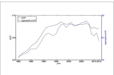
This data set contains a small portion of the firms accounted for Japan GDP. The aggregate equity and aggregate profit contained in this data set are somehow related to the dynamic pattern of Japan GDP, see Figure 1 for the dynamics of aggregate equity and GDP and Figure 2 for the dynamics of aggregate profit and GDP.2

1

One can consider the dynamic projection for the future periodt+t′, which is equivalent to the dynamic projection for the next periodt+1 byt′times.

2_{The data source for Japan GDP is obtained from the World Bank. The link to the data is:}

1980 1985 1990 1995 2000 2005 2010 2012 222

399 576

GDP

year

1980 1985 1990 1995 2000 2005 2010 201224

123 222

aggregate equity

GDP

aggregate equity

Figure 1: Aggregate equity and Japan GDP (in Trillion Yen).

3.4

Dynamic Projection of Aggregate Equity

By Equation (6), the dynamic projection of aggregate equity requires the quantifi-cation of the aggregation in micro-level firms equity and the transition matrix based on firms equity level. Specifically, at the end of yeart, we have by computation the following data:

1. The number of binsN =10 by setup;3

2. The distribution of the firms equity structure at yeart: frs[t] = (f r[s1,t],. . .,

f r[sN,t]);

3. The transition matrix computed by Equation (4) at the end of yeart:M[t−1]; 4. The average equity level for each binsn[t],n= 1, . . . ,N at yeart, denoted in

vector form:AS[t]=(A1[t], . . . ,An[t],. . .,AN[t]).

Suppose “as-if” the economy,ceteris paribus, from periodtto periodt+1. By Equation 5, the aggregation of meso-level structural change at next yeart+1 is estimated as: frcs[t+1|t] = frs[t]·M[t−1]. The aggregation in micro-level firms

equity at next yeart+1 is estimated byAS[t], the average equity level for each bin

3

1980 1985 1990 1995 2000 2005 2010 2012 222

399 576

GDP

year

1980 1985 1990 1995 2000 2005 2010 201222

51 80

aggregate profit

GDP

aggregate profit

Figure 2: Aggregate profit and Japan GDP (in Trillion Yen).

at yeart. With the notation< , >for scalar product, the one-period-ahead dynamic projection of aggregate equity at yeartfor yeart+1 is formulated as:

c

DP(A)t+1|t =< cfrs[t+1|t],AS[t]>=< frs[t]·M[t−1],AS[t]> . (7)

c

DP(A)t+1|t can be regarded as one-period-ahead out-of-sample forecast of

the aggregate equity computed at year t for year t+ 1. To testify its forecasting performance, we split the data set into two halves, with the first half as the training set that contains 17 annual data for the year of 1980 to 1996 and the second half as the target set that contains 16 annual data for the year of 1997 to 2012. We compare the one-period-ahead out-of-sample forecast by dynamic projection with the benchmark of the classical ARIMA model on the aggregate equity at the year of 1997 to 2012.

We use the aggregate equity for the year 1980 to 1996 as the initial infor-mation set for ARIMA model. At the end of each year t = 1996, . . . ,2011, use the up-to-date information set on aggregate equity. For example, at the end of year

aggre-gate equity, denoted as:

d

ARI MA(A)t+1|t ={ARI MAd (A)1997|1996, . . . ,ARI MAd (A)2012|2011}. (8)

Then compare with the dynamic projectionDPc(A)t+1|t ={DPc(A)1997|1996,. . ., c

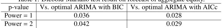
DP(A)2012|2011}, by applying Diebold-Mariano test with linear loss function (power =1) and quadratic loss function (power = 2). We construct the null hypothesis: ARIMA method has at least the same forecast accuracy as the dynamic projection on aggregate equity. The alternative hypothesis is thus: ARIMA is less accurate than dynamic projection on aggregate equity. Table 1 shows the p-value for the comparison with optimal ARIMA on BIC and on AICc information criterion with linear loss function and quadratic loss function.

Table 1: Diebold-Mariano test result on forecast of aggregate equity. p-value Vs. optimal ARIMA with BIC Vs. optimal ARIMA with AICc

Power=1 0.036 0.028

Power=2 0.042 0.029

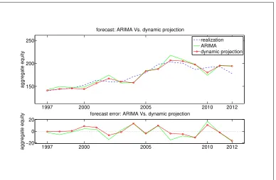
The p-values shown in Table 1 indicate that we reject the null hypothesis with 95% confidence, and accept the alternative hypothesis that dynamic projection for aggregate equity has higher forecasting accuracy than optimal ARIMA with BIC and AICc information criterion. As a visualization, Figure 3 shows in the upper plot the dynamics of the actual time series of aggregate equity for the year 1997 to 2012 (blue line), the dynamic projection (red line), and the optimal ARIMA with BIC information criterion (green line). It shows in the lower plot the forecast error for the dynamic projection (red line) and that for the optimal ARIMA (green line).

3.5

Dynamic Projection of Aggregate Profit

We consider the firms profit is related to the stock variable of firms equity level. By Equation (6), the dynamic projection of aggregate profit hence requires the quantifi-cation of the aggregation in micro-level firms profit and the transition matrix based on firms equity structure. Specifically, at the end of yeart, we have by computation the following data:

1. The number of binsN =10 by setup;4

2. The distribution of the firms equity structure at yeart: frs[t] = (f r[s1,t],. . .,

f r[sN,t]);

4

1997 2000 2005 2010 2012 150

200 250

aggregate equity

forecast: ARIMA Vs. dynamic projection

realization ARIMA

dynamic projection

1997 2000 2005 2010 2012

−20 0 20

aggregate equity

forecast error: ARIMA Vs. dynamic projection

Figure 3: Forecast for aggregate equity: ARIMA Vs. dynamic projection (in Tril-lion Yen).

3. The transition matrix computed by Equation (4) at the end of yeart:M[t−1]; 4. The average profit for each binsn[t],n=1, . . . ,N at yeart, denoted in vector

form:_ΠS[t]=(Π1[t],. . .,ΠN[t]).

Suppose “as-if” the economy,ceteris paribus, from periodtto periodt+1. By Equation 5, the aggregation of meso-level structural change at next yeart+1 is estimated as: frcs[t+1|t] = frs[t]·M[t−1]. The aggregation in micro-level firms

profit at next yeart+1 is estimated byΠS[t], the average firm’s profit for each bin

at yeart. The one-period-ahead dynamic projection of aggregate profit at yeartfor yeart+1 is formulated as:

c

DP(Π)t+1|t =<frcs[t+1|t],ΠS[t]>=<frs[t]·M[t−1],ΠS[t]> . (9)

c

DP(Π)t+1|t can be regarded as one-period-ahead out-of-sample forecast of

the aggregate profit computed at year t for year t + 1. Analogously, we testify its forecasting performance, by comparing with the benchmark of the classical ARIMA model on the aggregate profit at the year of 1997 to 2012.

the up-to-date information set on aggregate profit. We also apply two information criteria, BIC and AICc, to choose the optimal ARIMA model to conduct the one-period-ahead out-of-sample forecast on aggregate profit, denoted as:

d

ARI MA(Π)t+1|t = {ARI MAd (Π)1997|1996, . . . ,ARI MAd (Π)2012|2011}. (10)

Then we compare with the dynamic projectionDPc(Π)t+1|t ={DPc(Π)1997|1996,

. . ., DPc(Π)2012|2011}, by applying Diebold-Mariano test with linear loss function

(power =1) and quadratic loss function (power = 2). We construct the null hy-pothesis: ARIMA method has at least the same forecast accuracy as the dynamic projection on aggregate profit. The alternative hypothesis is thus: ARIMA is less accurate than dynamic projection on aggregate profit. Table 2 shows the p-value for the comparison with optimal ARIMA on BIC and on AICc information criterion with linear loss function and quadratic loss function.

Table 2: Diebold-Mariano test result on forecast of aggregate profit. p-value Vs. optimal ARIMA with BIC Vs. optimal ARIMA with AICc

Power=1 0.014 0.022

Power=2 0.027 0.033

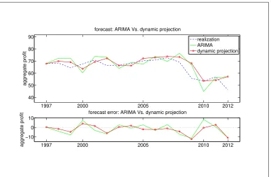
The p-values shown in Table 2 indicate that we reject the null hypothesis with 95% confidence, and accept the alternative hypothesis that dynamic projection for aggregate profit has higher forecasting accuracy than optimal ARIMA with BIC and AICc information criterion. As a visualization, Figure 4 shows in the upper plot the dynamics of the actual time series of aggregate profit for the year 1997 to 2012 (blue line), the dynamic projection (red line), and the optimal ARIMA with BIC information criterion (green line). It shows in the lower plot the forecast error for the dynamic projection (red line) and that for the optimal ARIMA (green line).

3.6

Sensitivity Analysis on Number of Bins

1997 2000 2005 2010 2012 40

50 60 70 80 90

aggregate profit

forecast: ARIMA Vs. dynamic projection

realization ARIMA

dynamic projection

1997 2000 2005 2010 2012

−10 0 10

aggregate profit

forecast error: ARIMA Vs. dynamic projection

Figure 4: Forecast for aggregate profit: ARIMA Vs. dynamic projection (in Trillion Yen).

Table 3 and Table 4 showp-values of Diebold-Mariano test with linear loss function (power=1) and quadratic loss function (power=2), forN = 2, . . . ,7 and

N =8, . . . ,13 respectively.

Table 3: Diebold-Mariano test results with number of binsN =2, . . . ,7

number of bins 2 3 4 5 6 7

BIC, power=1 0.049 0.045 0.024 0.034 0.037 0.056 aggregate BIC, power=2 0.087 0.069 0.036 0.059 0.041 0.092 equity AICc, power=1 0.040 0.038 0.018 0.027 0.029 0.040 AICc, power=2 0.065 0.051 0.025 0.042 0.029 0.065 BIC, power=1 0.007 0.014 0.007 0.015 0.017 0.021 aggregate BIC, power=2 0.016 0.015 0.006 0.018 0.021 0.033 profit AICc, power=1 0.008 0.020 0.012 0.022 0.027 0.033 AICc, power=2 0.019 0.019 0.008 0.022 0.027 0.040

Table 4: Diebold-Mariano test results with number of binsN = 8, . . . ,13

number of bins 8 9 10 11 12 13

BIC, power=1 0.023 0.074 0.036 0.049 0.038 0.185 aggregate BIC, power=2 0.039 0.109 0.042 0.062 0.048 0.175 equity AICc, power=1 0.016 0.055 0.028 0.037 0.025 0.117 AICc, power=2 0.026 0.078 0.029 0.044 0.032 0.109 BIC, power=1 0.010 0.033 0.014 0.042 0.041 0.061 aggregate BIC, power=2 0.010 0.056 0.027 0.091 0.039 0.060 profit AICc, power=1 0.016 0.045 0.022 0.061 0.061 0.085 AICc, power=2 0.014 0.065 0.033 0.104 0.047 0.070

ARIMA with BIC and AICc information criterion. The only two exceptions are on the scenario ofN = 9 for aggregate equity, against optimal ARIMA models under BIC criterion, where Diebold-Mariano test under quadratic loss function (power=

2) gives the p-value= 0.109; and on the scenario of N = 11 for aggregate profit, against optimal ARIMA models under AICc criterion, where Diebold-Mariano test under quadratic loss function (power=2) gives the p-value=0.104.

We may argue a potential explanation on the poor performance for N = 9 and N = 11 from the perspective of round-off error. For instance, for N = 9, we need to construct the bins sn[t] for n = 1, . . . ,9 by Equation (1), where sn[t]

equally contains 1₉ population of firms. In numerical computation, 1₉ can only be approximated by floating-point number with certain digits of rounding, i.e. 1₉ ≈

0.1111 under 4-digits of chopping or 1

9 ≈ 0.11 under 2-digits of chopping. In any

case of chopping, we face the round-off error for N = 9, which might not have insignificant impact on the computation. Similar situation happens forN =11.

Another observation from these two tables is that, for number of binsN =

13, the highest p-value is 0.185 > 0.10 for aggregate equity, while the highest p -value is 0.085>0.05 for aggregate profit. It shows no strong support with statistical significance that dynamic projection has higher forecasting accuracy than optimal ARIMA with BIC and AICc information criterion. This indicates that increasing the number of bins does not necessarily lead to better performance of dynamic projection. We conduct another tests with higher number of binsN = 14, . . . ,17, which gives us the highest p-value larger than 0.10 in general, with some scenarios even larger than 0.30.

These findings suggest us to selectN ∈ {2, . . . ,12}. Moreover, we prefer less impact from round-offerrors on computation, which suggests choosingN that less likely generates round-offerrors, i.e. _N1 can be exactly represented by floating-point number under finite digits. In this regard, we suggest a rule of thumb of choosing

4

Concluding Remark

Employing the viewpoint that economic system can be regarded as multi-level dy-namical system, we have developed in this paper a quantification on the meso-level structural change by applying the concept of transition matrix with appropriate par-tition on the micro-level state of the economic system. We have utilized this method of quantification to develop a technique of dynamic projection that can be used to compute out-of-sample forecasting of macro-level economic variable from micro-level Big Data. We have shown this technique of dynamic projection gives us poten-tial to project the future state of macro-level economic variable of aggregate equity and aggregate profit from the data set of firms listed in Tokyo Stock Exchange for the year of 1980 to 2012. In the coming era of Big Data, this technique can be re-garded as the building block for a Central Guidance System (CGS) to monitor and to guide the direction of the economy in a real-time manner.

In this paper, we have developed the technique of dynamic projection with-out the consideration of network topology among economic agents in the system. Since network structure can be represented by adjacency matrix that shares simi-larity to transition matrix, it is reasonable to believe the technique of dynamic pro-jection can be applied in this scenario, with the inclusion of adjacency matrix with transition matrix, which is left as one of the future tasks in our research agenda.

By our research, it seems that our construction of transition matrix works as an appropriate measurement and quantification on the meso-level structural change. It suggests, behind this finding, there might exist mathematical foundation for sup-porting and guiding us on developing technique on quantifying meso-level struc-tural change. Another future task is concerned with exploring the mathematical foundation in this sense.

In our work, we have shown the number of binsNthat defines the dimension of the transition matrix plays an important role in the technique of dynamic projec-tion. By statistical test, we have conducted sensitivity analysis of this key parameter on the performance of dynamic projection and have demonstrated the rule of thumb on how to chooseN. We expect a more comprehensive analysis from mathematical perspective on this topic in our future study, in relation with information theory and statistical mechanics.

References

Aoki, M. (2004): Modeling aggregate behavior and fluctuations in economics: stochastic views of interacting agents, Cambridge University Press.

Aoki, M. and H. Yoshikawa (2011): Reconstructing macroeconomics: a perspec-tive from statistical physics and combinatorial stochastic processes, Cambridge University Press.

Battiston, S., D. Delli Gatti, M. Gallegati, B. Greenwald, and J. E. Stiglitz (2012): “Liaisons dangereuses: Increasing connectivity, risk sharing, and systemic risk,”

Journal of Economic Dynamics and Control, 36, 1121–1141.

Bianchi, F. (2012): “Regime switches, agents’ beliefs, and post-world war ii u.s. macroeconomic dynamics,”The Review of Economic Studies.

Chen, X. and R. Macdonald (2012): “Realized and Optimal Monetary Policy Rules in an Estimated MarkovSwitching DSGE Model of the United Kingdom,” Jour-nal of Money, Credit and Banking, 44, 1091–1116.

Davig, T. and E. M. Leeper (2005): “Generalizing the taylor principle,” Technical report, National Bureau of Economic Research.

Davig, T. and E. M. Leeper (2008): “Endogenous monetary policy regime change,” inNBER International Seminar on Macroeconomics 2006, University of Chicago Press, 345–391.

Delli Gatti, D., M. Gallegati, B. C. Greenwald, A. Russo, and J. E. Stiglitz (2012): “Mobility constraints, productivity trends, and extended crises,”Journal of Eco-nomic Behavior&Organization, 83, 375–393.

Diebold, F., J.-H. Lee, and G. Weinbach (1994): “Regime switching with time-varying transition probabilities,” in C. Hargreaves, ed.,Nonstationary Time Se-ries Analysis and Cointegration, Advanced Texts in Econometrics, Oxford Uni-versity Press, 283–302.

Engel, C. and J. D. Hamilton (1990): “Long Swings in the Dollar: Are They in the Data and Do Markets Know It?”American Economic Review, 80, 689–713. Foerster, A. (2013): “Monetary policy regime switches and macroeconomic

dy-namics,” 2013 Meeting Papers 906, Society for Economic Dynamics.

Foley, D. K. (1994): “A statistical equilibrium theory of markets,”Journal of Eco-nomic Theory, 62, 321–345.

Garcia, R. and P. Perron (1996): “An analysis of the real interest rate under regime shifts,”The Review of Economics and Statistics, 111–125.

Gintis, H. (2013): “Markov models of social dynamics: theory and applications,”

ACM Transactions on Intelligent Systems and Technology (TIST), 4, 53.

Goodwin, T. H. (1993): “Business-cycle analysis with a markov-switching model,”

Journal of Business&Economic Statistics, 11, 331–339.

Kim, C.-J. and C. R. Nelson (1998): “Business Cycle Turning Points, A New Co-incident Index, And Tests Of Duration Dependence Based On A Dynamic Factor Model With Regime Switching,” The Review of Economics and Statistics, 80, 188–201.

Kirman, A. P. (2011): Complex economics : individual and collective rationality, Routledge London.

Landini, S., M. Gallegati, and J. Stiglitz (2014a): “Economies with heterogeneous interacting learning agents,”Journal of Economic Interaction and Coordination, 1–28.

Landini, S., M. Gallegati, J. E. Stiglitz, X. Li, and C. Di Guilmi (2014b): “Learning and macro-economic dynamics,”Nonlinear Economic Dynamics and Financial Modelling, Essays in Honour of Carl Chiarella.

Liu, Z., D. F. Waggoner, and T. Zha (2011): “Sources of macroeconomic fluctu-ations: A regimeswitching DSGE approach,” Quantitative Economics, 2, 251– 301.

Lux, T. (2008): “Applications of statistical physics in finance and economics,” Technical report, Kieler Arbeitspapiere.

Pfante, O., N. Bertschinger, E. Olbrich, N. Ay, and J. Jost (2013): “Comparison between different methods of level identification,”Advances in Complex Systems, submitted.

Riccetti, L., A. Russo, and M. Gallegati (2014): “An agent based decentralized matching macroeconomic model,”Journal of Economic Interaction and Coordi-nation, 1–28.

Sims, C. A., D. F. Waggoner, and T. Zha (2008): “Methods for inference in large multiple-equation markov-switching models,” Journal of Econometrics, 146, 255–274.