Greedy Transition Based Dependency Parsing with Stack LSTMs

Parsing with Stack LSTMs

Miguel Ballesteros

IBM T. J. Watson Research Center

Chris Dyer

Carnegie Mellon University

Yoav Goldberg

Noah A. Smith

We introduce a greedy transition-based parser that learns to represent parser states using recurrent neural networks. Our primary innovation that enables us to do this efficiently is a new control structure for sequential neural networks—the stack long short-term memory unit (LSTM). Like the conventional stack data structures used in transition-based parsers, elements can be pushed to or popped from the top of the stack in constant time, but, in addition, an LSTM maintains a continuous space embedding of the stack contents. Our model captures three facets of the parser’s state: (i) unbounded look-ahead into the buffer of incoming words, (ii) the complete history of transition actions taken by the parser, and (iii) the complete contents of the stack of partially built tree fragments, including their internal structures. In addition, we compare two different word representations: (i) standard word vectors based on look-up tables and (ii) character-based models of words. Although standard word embedding models work well in all languages, the character-based models improve the handling of out-of-vocabulary words, particularly in morphologically rich languages. Finally, we discuss the use of dynamic oracles in training the parser. During training, dynamic oracles alternate between sampling parser states from the training data and from the model as it is being learned, making the model more robust to the kinds of errors that will be made at test time. Training our model with dynamic oracles yields a linear-time greedy parser with very competitive performance.

∗IBM T. J. Watson Research Center, 1101 Kitchawan Road, Route 134, Yorktown Heights, NY 10598. E-mail:[email protected].

∗∗Language Technologies Institute, Carnegie Mellon University, 5000 Forbes Avenue, Pittsburgh, PA 15213, USA. E-mail:[email protected] affiliated with DeepMind, London, UK.

†Computer Science Department, Bar-Ilan University, Ramat Gan, 5290002 Israel. E-mail:[email protected].

‡Computer Science & Engineering, University of Washington, Box 352350, Seattle, WA 98195, USA. E-mail:[email protected].

1 This work was done while Miguel was at Universitat Pompeu Fabra and Carnegie Mellon University. Submission received: 16 September 2015; revised version received: 6 April 2016; accepted for publication: 14 June 2016.

1. Introduction

Natural language parsing can be formulated as a series of decisions that read words in sequence and incrementally combine them to form syntactic structures; this formulation is known as transition-based parsing, and is often coupled with a greedy inference procedure (Yamada and Matsumoto 2003; Nivre 2003, 2004, 2008). Greedy transition-based parsing is attractive because the number of operations required to build any projective parse tree is linear in the length of the sentence, making greedy versions of transition-based parsing computationally efficient relative to graph- and grammar-based alternative formalisms, which usually require solving superlinear search prob-lems. The challenge in transition-based parsing is modeling which action should be taken in each of the states encountered as the parsing algorithm progresses.2

Because the parser state involves the complete sentence—which is unbounded in length—the representational challenge faced by the modeler is to find a finite encoding of an infinite space. This challenge is usually dealt with by making assumptions about state equivalence by selecting features of the state believed by the model-builder to be most informative (e.g., the next three words in the sequence, the roots of the two most recently built subtrees and their left- and right-most children, and so on).3

In this article, we advocate a recursive approach, in which complex parser states are represented as the composition of simpler ones, and these are constructed incrementally as parsing proceeds. Thus, we operate in a paradigm in which the model builder de-signs recursive architectures that automatically discover effective views of the complete parser’s evolving state rather than explicitly engineering which features of the state to focus on. This construction enables us to avoid making explicit state-equivalence as-sumptions. We present one such architecture based on advances in recursively defined neural networks. Our state representation integrates information from a wide range of sources:

r

r

r

structures.

This global sensitivity of the state representation contrasts with most previous work in transition-based parsing that considers only a “narrow view” of the parser state when extracting features used to predict actions. Our work is complementary to previous approaches that develop alternative transition operations to simplify the modeling problem and enable better attachment decisions (Nivre 2007, 2008, 2009; Bohnet and Nivre 2012; Choi and McCallum 2013) and to feature engineering (Zhang and Nivre 2011; Ballesteros and Bohnet 2014; Chen, Zhang, and Zhang 2014; Ballesteros and Nivre 2016).

Our model is related to recent work that uses neural networks in dependency parsing (Chen and Manning 2014; Weiss et al. 2015; Zhou et al. 2015; Andor et al. 2016).

2 The term “state” refers to the collection of previous decisions (sometimes called the history), resulting partial structures, which are stored in a stack data structure, and the words remaining to be processed. 3 These state equivalence assumptions are similar to the Markov assumptions made in modeling stochastic

That work can broadly be understood as replacing a conventional linear classifier with a neural network classifier but still only considering a “narrow view” of the parser state, whereas our work uses recursively defined networks to incorporate sensitivity to the complete parser state.

Using recursive/recurrent neural networks to compute representations of un-boundedly large histories has been proposed previously (Henderson 2003; Titov and Henderson 2007b; Stenetorp 2013; Yazdani and Henderson 2015). Our innovation is to make the architecture of the neural network identical with the structure of stack data structures used to store the parser state. To do so, the technical challenge we must solve is being able to access, in constant time, a fixed-size representation of a stack as it evolves during the course of parsing. The technical innovation that lets us do this is a variation of recurrent neural networks with long short-term memory units (LSTMs), which we callstack LSTMs(Section 2). These can be understood as LSTMs augmented with a stack pointer that is manipulated by push and pop operations (in contrast to classic LSTMs that only ever read inputs sequentially).

Our parsing model uses three stack LSTMs to construct the parser state represen-tation: one containing the unprocessed input tokens, one containing the stack of partial syntactic trees, and one containing the history of parse actions (Section 3). Because the stack of partial syntactic trees may contain both individual tokens and partial syntactic structures, representations of individual tree fragments are computed compositionally with recursive neural networks, similar to Paulus et al. (2014).

The parser depends on vector representations of word tokens. Such representa-tions are most commonly learned as a dictionary lookup function (i.e., a map of each word type to a vector), but they can take a parameterized form that is, for example, sensitive to orthographic or morphological properties of a word’s surface form (Botha and Blunsom 2014). For languages with rich inflective morphology, surface clues can be quite helpful for parsing (Ballesteros 2013). In Section 4, we compare the classical lookup-table approach to a recently proposed model that combines representations of individual characters (using sequential LSTMs) to obtain a representation of the word. With no explicit morphological annotation, we find that the latter representation gives a large performance increase when parsing Statistical Parsing of Morphologically Rich Languages (SPMRL) data sets in languages with agglutinative morphology or extensive case systems (Seddah et al. 2013; Seddah, K ¨ubler, and Tsarfaty 2014), and performs as well as the table method in analytic languages. We further find that, without part-of-speech tags, this technique benefits all languages, and that in some cases this approach obviates the need for explicit part-of-speech information.

This article is an extension of publications by Dyer et al. (2015) and Ballesteros et al. (2015). It contains a more detailed background about LSTMs and parsing, a discussion about the effect of random initialization, more extensive experiments with standard data sets, experiments including explicit morphological information that yields much higher results than the ones reported before, and a new training algorithm following dynamic oracles that yield state-of-the-art performance while maintaining a fast parsing speed with a greedy model. An open-source implementation of our parser, in all its different instantiations, is available from

https://github.com/clab/lstm-parser.

2. Stack LSTMs

In this section we provide a review of LSTMs (Section 2.1), the core component of our parsing algorithm, and then define stack LSTMs (Section 2.2).

Notation. We follow the convention that vectors are written with lowercase, boldface letters (e.g.,vorvw); matrices are written with uppercase, boldface letters (e.g.,M,Ma, orMab), and scalars are written as lowercase letters (e.g.,sorqz). Structured objects such as sequences of discrete symbols are written with lowercase, bold, italic letters (e.g.,w refers to a sequence of input words). We use a semicolon to denote vector concatena-tion (e.g., [a;b]). Discussion of dimensionality is deferred to the experiments section (Section 6).

2.1 Long Short-Term Memories

Recurrent neural networks (RNNs) are non-linear functions from vector sequences to vector sequences. The term “recurrent” evokes the iterative application of the same function, given each prefix of the input, to calculate a “hidden state” vector. Con-cretely, let xt be the tth input vector and ht be the tth state vector. The incremental calculation is:

ht=σ(Wxxt+Whht−1+d)

Wx∈Rdout×din W

h ∈Rdout×dout _d,h

t∈Rdout _x

t∈Rdin

That is, the vectorxtis “read” in and a linear map is applied to it alongside the previ-ous state vectorht−1, then passed through a nonlinear function (here, a component-wise

logistic sigmoid, denotedσ). The state may then be further transformed to produce an output, either at each timestep or just at the end of the sequence.

The parameters of the RNN—here,Wx,Wh, andd—are estimated to minimize a loss function on the training data. The gradient for this loss tends to “vanish” (go to zero) as we trace it back to earlier iterates in a long sequence. This means that long-range dependencies along the input sequence are hard to capture in a learned RNN (Bengio, Simard, and Frasconi 1994).

the memory cell (it) and what proportion of the previous memory cell to “forget” (ft). The updated value of the memory cell after an inputxtis computed as follows:

it=σ(Wixxt+Wihht−1+Wicct−1+di)

ft=1−it

ct=ftct−1+ittanh(Wcxxt+Wchht−1+dc)

whereis the component-wise (Hadamard) product. The valuehtof the LSTM at each timestep is controlled by a third gate (ot) that is applied to the result of the application of a nonlinearity to the memory cell contents:

ot=σ(Woxxt+Wohht−1+Wocct+do) ht=ottanh(ct)

W◦x∈Rdout×din W

◦h,W◦c∈Rdout×dout _i

t,ft,ct,ot,ht,d◦∈Rdout _x

t∈Rdin

Note that our formulation differs slightly from the classic LSTM formulation in that it makes use of “peephole connections” that connect both cell values (thecs) and hidden states (the hs) to the gates (Gers, Schraudolph, and Schmidhuber 2003) and that it defines the forget gate so that it sums with the input gate to1(Greff et al. 2015).

To improve the representational capacity of LSTMs (and RNNs generally), LSTMs can be stacked in “layers” (Pascanu et al. 2013). In these architectures, the input LSTM at higher layers at timetis the value ofhtcomputed by the lower layer (andxtis the input at the lowest layer).

Finally, output is produced at each timestep from thehtvalue at the top layer: yt=g(ht)

yt,ht∈Rdout

where g is an arbitrary differentiable function. We use the identity function in this article.

2.2 Stack Long Short-Term Memories

Conventional LSTMs model sequences in a left-to-right order.4 _{Our innovation is to}

augment the LSTM with a “stack pointer.” Like a conventional LSTM, new inputs are always added in the right-most position, but in stack LSTMs, the current location of the stack pointer determines which cell in the LSTM provides ct−1 and ht−1 when

computing the new memory cell contents.

In addition to adding elements to the end of the sequence, the stack LSTM provides apopoperation that moves the stack pointer to the previous element (i.e., the previous element that was extended, not necessarily the next-right-most element). Thus, the

;

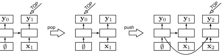
x

y

y

;

x

y

y

pop

;

x

y

y

TOP TOP

push

y

x

Figure 1

A stack LSTM extends a conventional left-to-right LSTM with the addition of a stack pointer (notated asTOPin the figure). This figure shows three configurations: a stack with a single element (left), the result of apopoperation to this (middle), and then the result of applying apush operation (right). The boxes in the lowest rows represent stack contents, which are the inputs to the LSTM, the upper rows are the outputs of the LSTM (in this article, only the output pointed to byTOPis ever accessed), and the middle rows are the memory cells (thects andhts) and gates.

Arrows represent function applications (usually affine transformations followed by a nonlinearity); refer to Section 2.1 for specifics.

LSTM can be understood as a stack implemented so that contents are never overwritten; that is,pushalways adds a new entry at the end of the list that contains a back-pointer to the previous top, andpop only updates the stack pointer.5 _{This control structure is}

schematized in Figure 1.

By querying the output vector to which the stack pointer points (i.e., hTOP), a

continuous-space “summary” of the contents of the current stack configuration is avail-able. We refer to this value as the “stack summary.” Note that this structure allows a given sequence history to have various different “continuations” that are independent from each other but are all linked to the same history. Signals from each continuation can then be backpropagated to the same shared history. Although elements near the top of the stack are likely to influence the stack summary the most, the LSTM has additional flexibility allowing it to learn to extract information from arbitrary points in the stack (Hochreiter and Schmidhuber 1997).

Although this architecture is novel, it is closely related to the recurrent neural network pushdown automaton of Das et al. (1992), which added an external stack memory to an RNN; the continuous stack transducers of Grefenstette et al. (2015); or the one proposed by Joulin and Mikolov (2015). Our formulation preserves the discrete pushandpopoperations of conventional stack data structures, whereas prior work uses continuous-valued relaxations of these.

3. Dependency Parser

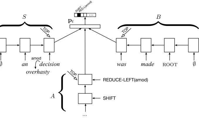
We now turn to the problem of learning representations of dependency parser states. We preserve the standard data structures of a transition-based dependency parser, namely, a buffer of words to be processed (B) and a stack (S) of partially constructed syntactic elements. Each stack element is augmented with a continuous-space vector embedding representing a word and, in the case ofS, any of its syntactic dependents. Additionally, we introduce a third stack (A) to represent the history of transition actions taken by the

overhasty

an decision was

amod

REDUCE-LEFT(amod)

SHIFT

|

{z

}

}

{z

|

|

{z

}

…

SHIFTRED-L(amod)

…

made

S B

A

; ;

pt

root TOP

TOP

TOP

Figure 2

Parser state computation encountered while parsing the sentencean overhasty decision was made. HereSdesignates the stack of partially constructed dependency subtrees and its LSTM encoding;

Bis the buffer of words remaining to be processed and its LSTM encoding; andAis the stack representing the history of actions taken by the parser. These are linearly transformed, passed through a rectified linear unit nonlinearity to produce the parser state embeddingpt. An affine transformation of this embedding is passed to a softmax layer to give a distribution over parsing decisions that can be taken.

parser.6Each of these stacks is associated with a stack LSTM that provides an encoding of its current contents. The full architecture is illustrated in Figure 2, and we will review each of the components in turn.

3.1 Parser Operation

The dependency parser is initialized by pushing the words and their representations (we discuss word representations in Section 4) of the input sentence in reverse order onto B such that the first word is at the top of B and the ROOT symbol is at the bottom, andSandAeach contain an empty-stack token. At each timestep, the parser computes a composite representation of the stack states (as determined by the current configurations ofB,S, andA) and uses that to predict an action to take, which updates the stacks. Processing completes whenBis empty (except for the empty-stack symbol),S contains two elements, one representing the full parse tree headed by theROOTsymbol and the other the empty-stack symbol,7 and Ais the history of transition operations taken by the parser.

6 TheAstack is only ever pushed to; our use of a stack here is purely for implementational and expository convenience.

The parser state representation at time t, which we write pt, which is used to determine the transition to take, is defined as follows:

pt=max{0,W[st;bt;at]+d}

st,bt,at∈Rdout p

t,d∈Rdstate _W∈

Rdstate×3dout

whereWis a learned parameter matrix,dis a learned bias term, andbt,st, andatare the stack LSTM encodings ofB,S, andA, respectively. These are then passed through a component-wise rectified linear unit (ReLU) nonlinearity (Glorot, Bordes, and Bengio 2011).8

Finally, the parser statept is used to compute the probability of the parser action at timetas:

p(zt|pt)=

exp g>_ztpt+qzt P

z0_∈A(S,B)exp g>_z0p_t+q_z0 (1)

pt,gz∈Rdstate

wheregz is a column vector representing the (output) embedding of the parser action z, and qz is a bias term for action z. The set A(S,B) represents the valid transition actions that may be taken given the current contents of the stack and buffer.9_Because

pt=f(st,bt,at) encodes information about all previous decisions made by the parser, the chain rule may be invoked to write the probability of any valid sequence of parse transitionszconditional on the input as:

p(z|w)= |z| Y

t=1

p(zt|pt) (2)

3.2 Composition Functions

Recursive neural network models enable complex phrases to be represented composi-tionally in terms of their parts and the relations that link them (Hermann and Blunsom 2013; Socher et al. 2011, 2013a, 2013b). We follow previous work in embedding depen-dency tree fragments that are present in the stackSin the same vector space as the token embeddings discussed in Section 4.

A particular challenge here is that a syntactic head may, in general, have an arbitrary number of dependents. To simplify the parameterization of our composition function, we combine head-modifier pairs one at a time, building up more complicated structures

8 In preliminary experiments, we tried several nonlinearities and found ReLU to work slightly better than the others.

decision

overhasty

an

overhasty

decision

an

c

mod _head

head mod

amod amod

c

rel

c

det rel

Figure 3

The representation of a dependency subtree (top) is computed by recursively applying

composition functions tohhead, modifier, relationitriples. In the case of multiple dependents of a single head, the recursive branching order is imposed by the order of the parser’s reduce transition (bottom).

in the order they are “reduced” in the parser, as illustrated in Figure 3. Each node in this expanded syntactic tree has a value computed as a function of its three arguments: the syntactic head (h), the dependent (m), and the syntactic relation being satisfied (r). We define this by concatenating the vector embeddings of the head, dependent, and relation and applying a linear operator and a component-wise nonlinearity as follows:

c=tanh (U[h;m;r]+e)

c,e,h,m∈Rdin _r∈

Rdrel _U∈

Rdin×(2din+drel)

For the relation vector, we use an embedding of the parser action that was applied to construct the relation (i.e., the syntactic relation paired with the direction of attachment); Uandeare additional parameters learned alongside those of the stack LSTMs.

3.3 Transition Systems

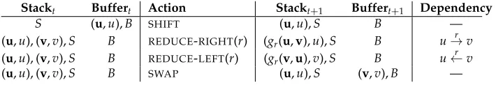
Our parser implements various transition systems. The original version (Dyer et al. 2015) implements arc-standard (Nivre 2004) in its most basic set-up. In Ballesteros et al. (2015), we augmented the arc-standard system with theSWAPtransition of Nivre (2009), allowing for nonprojective parsing. For the dynamic oracle training strategy, we moved to an arc-hybrid system (Kuhlmann, G ´omez-Rodr´ıguez, and Satta 2011) for which an efficient dynamic oracle is available. It is worth noting that the stack LSTM parameterization is mostly orthogonal to the transition system being used (providing that the system can be expressed as operating on stacks), making it easy to substitute transition systems.

3.3.1 Arc-Standard. The arc-standard transition inventory (Nivre 2004) is given in Figure 4. The SHIFT transition moves a word from the buffer to the stack, and the

Stackt Buffert Action Stackt+1 Buffert+1 Dependency

S (u,u),B SHIFT (u,u),S B —

(u,u), (v,v),S B REDUCE-RIGHT(r) (gr(u,v),u),S B u→r v

(u,u), (v,v),S B REDUCE-LEFT(r) (gr(v,u),v),S B u←r v

(u,u), (v,v),S B SWAP (u,u),S (v,v),B —

Figure 4

Parser transitions of thearc-standardsystem (with swap, Section 3.3.2) indicating the action applied to the stack and buffer and the resulting stack and buffer states. Bold symbols indicate (learned) embeddings of words and relations, script symbols indicate the corresponding words and relations. (gr(x,y),x) refers to the composition function presented in 3.2.

the stack. The arc-standard system allows building all and only projective trees. In order to parse nonprojective trees, this can be combined with the pseudo-projective approach (Nivre and Nilsson 2005) or follow what is presented in Section 3.3.2.

3.3.2 Arc-Standard with Swap. In order to deal with nonprojectivity, the arc-standard system can be augmented with a SWAP transition (Nivre 2009). TheSWAP transition removes the second-to-top item from the stack and pushes it back to the buffer, allowing for the creation of nonprojective trees. We only use this transition when the training data set contains nonprojective trees. The inclusion of theSWAPtransition requires breaking the linearity of the stack by removing tokens that are not at the top of the stack; however, this is easily handled with the stack LSTM. Figure 4 shows how the parser is capable of moving words from the stack (S) to the buffer (B), breaking the linear order of words. Because a node that is swapped may have already been assigned as the head of a dependent, the buffer (B) can now also contain tree fragments.

3.3.3 Arc-Hybrid.For the dynamic oracle training scenario, described in Section 5.2, we switch to the arc-hybrid transition system, which is amenable to an efficient dynamic oracle (Goldberg and Nivre 2013). The arc-hybrid system is summarized in Figure 5. The SHIFT and REDUCE-RIGHT transitions are the same as in arc-standard. However, theREDUCE-LEFTtransition pops the top of the stack and attaches it as a child of the first item in the buffer. Although it is possible to extend the arc-hybrid system to support nonprojectivity by adding aSWAPtransition, this extension would invalidate an important guarantee enabling efficient dynamic oracles.10 We therefore restrict the dynamic-oracle experiments to the fully projective English and Chinese treebanks. In order to parse nonprojective trees, this can be combined with the pseudo-projective approach (Nivre and Nilsson 2005).

4. Word Representations

Our parser’s architecture makes heavy use of word representations. We describe two variants. The first is a “standard” approach in which each word is represented

Stackt Buffert Action Stackt+1 Buffert+1 Dependency

S (u,u),B SHIFT (u,u),S B —

(u,u), (v,v),S B REDUCE-RIGHT(r) (gr(u,v),u),S B u r →v

(u,u),S (v,v),B REDUCE-LEFT(r) S (gr(v,u),v),B u←r v

Figure 5

Parser transitions of the arc-hybrid system (Section 3.3.3).Boldsymbols indicate (learned) embeddings of words and relations, italic symbols indicate the corresponding words and relations. (gr(x,y),x) refers to the composition function presented in 3.2.

as a vector, which is pretrained on unannotated data (Section 4.1). The second is a character-based representation, in which the word’s representation is highly depen-dent on its orthography. These character-based representations are trained without additional resources and work well for implicitly capturing the morphology of words (Section 4.2).

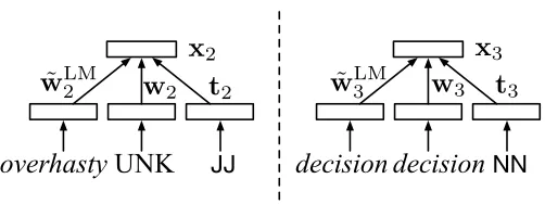
4.1 Standard Word Representations

To represent each input token, we concatenate three vectors: a learned vector repre-sentation for each word type (w), a fixed vector representation from a neural language model ( ˜wLM), and a learned representation (t) of the POS tag of the token, provided as

auxiliary input to the parser. A linear map (V) is applied to the resulting vector and passed through a component-wise ReLU:

x=max{0,V[w; ˜wLM;t]+d}

x,d∈Rdin w∈Rdword w˜LM ∈Rdlm t∈Rdpos V∈Rdin×(dword+dlm+dpos)

This mapping can be shown schematically as in Figure 6.

If there are morphological features available, containing information about gender, number or case, then we can also concatenate with a fourth vector that is a learned

overhasty

UNK

JJ

decision

decision

NN

x

x

t

t

w

˜

w

w

˜

w

Figure 6

representation (f) of the morphological tags of the token, again provided as auxiliary input to the parser. The linear map (V) would then be:

x=max{0,V[w; ˜wLM;t;f]+d}

x,d∈Rdin w∈Rdword w˜LM∈Rdlm t∈Rdpos f∈Rdmorph

V∈Rdin×(dword+dlm+dpos+dmorph)

This representation lets us deal flexibly with out-of-vocabulary (OOV) words— those that are OOV in the very limited parsing data but present in the pretraining language model (LM), and words that are OOV in both. To ensure we have estimates of the OOVs in the parsing training data, we stochastically replace (with probability 0.5) each singleton word type in the parsing training data with the UNK token in each training iteration.

Pretrained Word Embeddings.There are several options for creating word embeddings, meaning numerous pretraining options for w˜LM are available. However, for

syn-tax modeling problems, embedding approaches that discard order perform less well (Bansal, Gimpel, and Livescu 2014); therefore, we used a variant of the skip n-gram model introduced by Ling et al. (2015a), named “structured skip n-gram,” where a different set of parameters is used to predict each context word depending on its position relative to the target word.

4.2 Modeling Characters Instead of Words

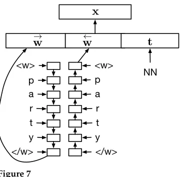
Following Ling et al. (2015b), we compute character-based continuous-space vector embeddings of words using bidirectional LSTMs (Graves and Schmidhuber 2005). When the parser initiates the learning process and populates the buffer with all the words from the sentence, it reads the words character by character from left to right and computes a continuous-space vector embedding the character sequence, which is theh vector of the LSTM; we denote it by−→w. The same process is also applied in reverse (albeit with different parameters), computing a similar continuous-space vector embedding starting from the last character and finishing at the first (←w−); again each character is represented with an LSTM cell. After that, we concatenate these vectors and a (learned) representation of their tag to produce the representationw. As in Section 4.1, a linear map (V) is applied and passed through a component-wise ReLU.

x=max0,V[−→w;←w−;t]+d

x,d∈Rdin −→w,←w−∈Rdout t∈Rdpos V∈Rdin×2dout+dpos

p

y a

r t y

t r a p

</w> <w>

</w> <w>

!

w

w

t

NN

x

Figure 7

Character-based word embedding of the wordparty. This representation is used for both in-vocabulary and out-of-vocabulary words.

As with the standard word representations, it is possible to concatenate with a fourth vector which is a learned representation (f) of the morphological tags of the token, again provided as auxiliary input to the parser:

x=max0,V[−→w;←w−;t;f]+d

x,d∈Rdin −→w,←w−∈Rdout t∈Rdpos f∈Rdmorph V∈Rdin×2dout+dpos+dmorph Note that under this representation, OOV words are treated as bidirectional LSTM encodings and thus they will be “close” to other words that the parser has seen during training, ideally close to their more frequent morphological relatives. We conjecture that this will give a clear advantage over a single “UNK” token for all the words that the parser does not see during training, as done in Section 4.1 and other parsers without additional resources. In Section 6 we confirm this hypothesis.

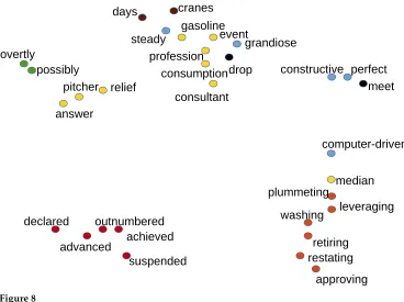
Learned Word Representations.Figure 8 visualizes a sample of the character-based bidi-rectional LSTMs learned representations (using the model referred to asCharsin Sec-tion 6.4). Clear clusters of past tense verbs, gerunds, and other syntactic classes are visible. The colors in the figure represent the most common POS tag for each word.

5. Training Procedure

The parser is trained to maximize the conditional probability of taking a “correct” action at each parsing state. (The definition of what constitutes a “correct” action is the major difference between static oracle and dynamic oracle training.) We begin with the simpler strategy of training with a static oracle (Section 5.1), then turn to dynamic oracles (Section 5.2).

overtly

possibly

declared

advanced

outnumbered

achieved

suspended

approving

restating

retiring

washing

leveraging

plummeting

median

computer-driven

cranes

days

steady

event

gasoline

grandiose

meet

perfect

constructive

drop

consumption

profession

consultant

relief

pitcher

answer

Figure 8

Character-based word representations of 30 random words from the English development set (Charsmodel; see Section 6.4). Dots in red represent past tense verbs; dots in orange represent gerund verbs; dots in black represent present tense verbs; dots in blue represent adjectives; dots in green represent adverbs; dots in yellow represent singular nouns; dots in brown represent plural nouns. The visualization was produced using t-SNE; seehttp://lvdmaaten.github.io/ tsne/.

section 4). The computations for a single parsing model were run on a single thread on a CPU. Using the dimensions discussed in the next section, we required between 8 and 12 hours to reach convergence on a held-out development set.11

5.1 Static Oracle Training

With a static oracle, the training procedure computes a canonical reference series of tran-sitions for each gold parse tree. It then runs the parser through this canonical sequence of transitions, while keeping track of the state representationptat each stept, as well as the distribution over transitionsp(zt|pt) that is predicted by the current classifier for the state representation. Once the end of the sentence is reached, the parameters are updated towards minimizing the cross-entropy of the reference transition sequence (Equation (2)) by minimizing the cross-entropy (i.e., maximizing the log-likelihood) of the correct transitionp(zt|pt) at each state along the path.

5.2 Training with Exploration using Dynamic Oracles

In the static oracle case, the parser is trained to predict the best transition to take at each parsing step, assuming all previous transitions were correct. Because the parser is likely to make mistakes at test time and encounter states it has not seen during training, this training criterion is problematic (Daum´e III, Langford, and Marcu 2009; Ross, Gordon, and Bagnell 2011; Goldberg and Nivre 2012, 2013, inter alia). Instead, we would prefer to train the parser to behave optimally also after making a mistake (under the constraints that it cannot backtrack or fix any previous decision). We thus need to include in the training examples states that result from wrong parsing decisions, together with the optimal transitions to take in these states. To this end we reconsider which training examples to show, and what it means to behave optimally on these training examples. The dynamic oracles framework for training with exploration, suggested by Goldberg and Nivre (2012, 2013), provides answers to these questions.

Although the application of dynamic oracle training is relatively straightforward, some adaptations were needed to accommodate the probabilistic training objective. These adaptations mostly follow Goldberg (2013).

5.2.1 Dynamic Oracles.Adynamic oracleis the component that, given a gold parse tree, provides the optimal set of possible actions to take under a given parser state. In contrast to static oracles that derive a canonical sequence for each gold parse tree and say nothing about parsing states that do not stem from this canonical path, the dynamic oracle is well-defined for states that result from parsing mistakes, and may produce more than a single gold action for a given state. Under the dynamic oracle framework, a parsing action is said to be optimal in a given state if the best tree that can be reached after taking the action is no worse (in terms of accuracy with respect to the gold tree) than the best tree that could be reached prior to taking that action.

Goldberg and Nivre (2013) define the arc-decomposition property of transition sys-tems, and show how to derive efficient dynamic oracles for transition systems that are arc-decomposable (see footnote 10). Unfortunately, the arc-standard transition system does not have this property. Although it is possible to compute dynamic oracles for the arc-standard system (Goldberg, Sartorio, and Satta 2014), the computation relies on a dynamic programming algorithm that is polynomial in the length of the stack. As the dynamic oracle has to be queried for each parser state seen during training, the use of this dynamic oracle will make the training times several times longer. We chose instead to switch to the arc-hybrid transition system (Kuhlmann, G ´omez-Rodr´ıguez, and Satta 2011), which is very similar to the arc-standard system but is arc-decomposable and hence admits an efficientO(1) dynamic oracle, resulting in only negligible burden on the training time. We implemented the dynamic oracle to the arc-hybrid system as described by Goldberg (2013).

predicted distribution, we are effectively increasing the chance of straying from the gold path during training, while still focusing on mistakes that receive relatively high parser scores. We believe further formal analysis of this method will reveal connections to reinforcement learning and, perhaps, other methods for learning complex policies.

Taking this idea further, we could increase the number of error-states observed in the training process by changing the sampling distribution so as to bias it toward more low-probability states. We do this by raising each probability to the power of

α (0< α_≤1) and re-normalizing. This transformation keeps the relative ordering of the events, while shifting probability mass towards less frequent events. As we show subsequently, this turns out to be very beneficial for the configurations that make use of external embeddings. Indeed, these configurations achieve high accuracies and shared class distributions early on in the training process.

The parser is trained to optimize the log-likelihood of a correct actionzg at each parsing statept according to Equation (1). When using the dynamic oracle, a statept may admit multiple correct actionszg={zgi,. . .,zgk}. Our objective in such cases is that the set of correct actions receives high probability. We optimize for the log ofp(zg|pt), defined as:

p(zg|pt)=

X

z_gi∈zg

p(zgi |pt) (3)

A similar approach was taken by Riezler et al. (2000), Charniak and Johnson (2005), and Goldberg (2013) in the context of log-linear probabilistic models.

6. Experiments

After describing the implementation details of our optimization procedure (Section 6.1) and the data used in our experiments (Section 6.2), we turn to four sets of experiments:

1. First, we assess the quality of our greedy, global-state stack LSTM parsers on a wide range of data sets, showing that it is highly competitive with the state of the art (Section 6.3).

2. We compare the performance of the two different word representations (Section 4) across different languages, finding that they are quite beneficial in some cases and harmless in most others (Section 6.4).

3. We compare dynamic oracles to static oracles, showing that training with dynamic oracles attains even better performance (Section 6.5).

4. We compare our parser with other existing methods on the CoNLL-2009 data sets (Section 6.6).

6.1 Optimization Procedure Details

Parameter optimization was performed using stochastic gradient descent with an ini-tial learning rate ofη₀=01; the learning rate was updated on each pass through the

(Graves 2013; Sutskever, Vinyals, and Le 2014). An`₂ penalty of 1×10−6was applied to all weights.

Matrix and vector parameters were initialized with uniform samples in

±p6/(r+c), where r and c were the number of rows and columns in the structure (Glorot and Bengio 2010). We use mini-batches of 1,000 sentences each and update every 25 iterations.

Dimensionality.The full version of our parsing model sets dimensionalities as follows. LSTM hidden states (dout) are of size 100, and we use two layers of LSTMs for each stack. Embeddings of the parser actions used in the composition functions (dstate) have 16 dimensions, and the output embedding (dout) size is 20 dimensions. Pretrained word embeddings (ddlm) have 100 dimensions (English) and 80 dimensions (Chinese), and the

learned word embeddings (dword) have 32 dimensions. Part of speech and morphological tag embeddings (dpos and dmorph) have 12 dimensions, when included. The character-based embeddings are of size 100, when included. The combined representations of the inputs have 100 dimensions.

These dimensions were chosen based on intuitively reasonable values (words should have higher dimensionality than parsing actions, POS tags, and relations; LSTM states should be relatively large), and it was confirmed on development data that they performed well.12Future work might more carefully optimize the parser’s hyperparam-eters. A variety of automated techniques have been developed for hyperparameter op-timization, including ones that enable evidence-sharing across related tasks (Yogatama and Mann 2014; Yogatama, Kong, and Smith 2015). Our architecture strikes a balance between minimizing computational expense and finding solutions that work.

Pretrained Word Vectors.The hyperparameters of the structured skipn-gram model are the same as in the skipn-gram model defined in the widely usedword2vec implemen-tation (Mikolov et al. 2013). We set the window size to 5, used a negative sampling rate to 10, and ran 5 epochs through unannotated corpora described in Section 6.2.

6.2 Data

We use different data depending on the targeted experiment; in this section we describe the data sets that we used to test the basic model, the character-based representations that are geared towards morphology, and the dynamic oracles. Finally, we also report results with the CoNLL 2009 data sets (Hajiˇc et al. 2009) to make a complete comparison with similar systems.

6.2.1 Data for the Simplest Model that Uses Word Representations and Static Oracle for Training.We used the same data set-up as Chen and Manning (2014), namely, an English task and a Chinese task. This baseline configuration was chosen because they likewise used a neural parameterization to predict actions in an arc-standard transition-based parser.

r

MacCartney, and Manning 2006) used in Chen and Manning (2014), which

is the closest model published, with the same splits.13_{The part-of-speech}

tags are predicted by using the Stanford POS tagger (Toutanova et al. 2003) with an accuracy of 97.3%. This treebank contains a negligible number of nonprojective arcs (Chen and Manning 2014).

r

Zhang and Clark (2008),14with gold part-of-speech tags, which is also the same as in Chen and Manning (2014).

Language model word embeddings were generated from the AFE portion of the English Gigaword corpus (version 5), and from the complete Chinese Gigaword corpus (version 2), as segmented by the Stanford Chinese Segmenter (Tseng et al. 2005).

6.2.2 Data to Test the Character-Based Representations and Static Oracle for Training.For the character-based representations we applied our model to the treebanks of the SPMRL Shared Task (Seddah et al. 2013; Seddah, K ¨ubler, and Tsarfaty 2014): Arabic (Maamouri et al. 2004), Basque (Aduriz et al. 2003), French (Abeill´e, Cl´ement, and Toussenel 2003), German (Seeker and Kuhn 2012), Hebrew (Sima’an et al. 2001), Hungarian (Vincze et al. 2010), Korean (Choi 2013), Polish (´Swidzi ´nski and Woli ´nski 2010), and Swedish (Nivre, Nilsson, and Hall 2006). For all the corpora of the SPMRL Shared Task, we used predicted POS tags as provided by the shared task organizers.15 We also ran the experiment with the Turkish dependency treebank16(Oflazer et al. 2003) of the CoNLL-X Shared Task (Buchholz and Marsi 2006) and we use gold POS tags when used as it is common with the CoNLL-X data sets. In addition to these, we include the English and Chinese data sets described in Section 6.2.1.

6.2.3 Data for the Dynamic Oracle.Because the arc-hybrid transition-based parsing algo-rithm is limited to fully projective trees, we use the same data as in Section 6.2.1, which makes it comparable with the basic model that uses standard word representations and a static oracle arc-standard algorithm.

6.2.4 CoNLL-2009 Data.We also report results with all the CoNLL 2009 data sets (Hajiˇc et al. 2009) to make a complete comparison with similar systems both for static and dynamic oracles.

6.3 Experiments with Static Oracle and Standard Word Representations

We report results on five experimental configurations per language, as well as the Chen and Manning (2014) baseline. These are: the full stack LSTM parsing model (S-LSTM), the stack LSTM parsing model without POS tags (−POS), the stack LSTM parsing model without pretrained language model embeddings (−pretraining), the

13 Training: 02-21. Development: 22. Test: 23.

14 Training: 001–815, 1001–1136. Development: 886–931, 1148–1151. Test: 816–885, 1137–1147. 15 The POS tags were calculated with MarMot tagger (Mueller, Schmid, and Sch ¨utze 2013) by the best

performing system of the SPMRL Shared Task (Bj ¨orkelund et al. 2013). Arabic: 97.38. Basque: 97.02. French: 97.61. German: 98.10. Hebrew: 97.09. Hungarian: 98.72. Korean: 94.03. Polish: 98.12. Swedish: 97.27.

Table 1

Unlabeled attachment scores and labeled attachment scores on thedevelopmentsets (top) and the finaltestsets (bottom) for Chinese and English (SD). The columns marked with S-LSTM show the results of the parser with the whole S-LSTM model. The columns marked with−POS show the results of the parser without POS tags. The columns marked with−pretraining show the results of the parser without pretraining. The columns marked with S-RNN show the results of the parser in which the S-LSTM is replaced by a recurrent neural network. The columns marked with C&M (2014) show the results of Chen and Manning (2014).

Development

S-LSTM −POS −pretraining −composition S-RNN C&M (2014)

Language UAS LAS UAS LAS UAS LAS UAS LAS UAS LAS UAS LAS

Chinese 87.23 85.87 82.65 79.84 85.96 84.37 86.32 84.59 86.30 84.70 84.0 82.4 English 93.11 90.80 92.58 89.96 92.58 90.24 92.50 89.79 92.80 90.40 92.2 89.7

Test

S-LSTM −POS −pretraining −composition S-RNN C&M (2014)

Language UAS LAS UAS LAS UAS LAS UAS LAS UAS LAS UAS LAS

Chinese 86.85 85.36 82.15 79.04 85.48 83.94 86.20 84.49 86.10 84.60 83.9 82.4 English 93.04 90.87 92.57 90.21 92.40 90.04 92.10 89.61 92.30 90.10 91.8 89.6

stack LSTM parsing model that uses just head words on the stack instead of com-posed representations (−composition), and the full parsing model where rather than an LSTM, a simple recurrent neural network in which normal sigmoidal hid-den units are used instead of the LSTM, but augmented with a stack pointer (S-RNN).

6.3.1 Results.Following Chen and Manning (2014), we exclude punctuation symbols for evaluation. Table 1 shows parsing scores comparable to Chen and Manning (2014),17 and we show that our model is better than their model on both the development set and the test set.

Overall, our parser substantially outperforms the baseline neural network parser of Chen and Manning (2014), both in the full configuration and in the various ablated conditions we report. The one exception to this is the−POS condition for the Chinese parsing task, in which we underperform their baseline (which used gold POS tags), although we do still obtain reasonable parsing performance in this limited case. We note that predicted POS tags in English add very little value—suggesting that we can think of parsing sentences directly without first tagging them. We also find that using composed representations of dependency tree fragments outperforms using representations of head words alone. Finally, we find that whereas LSTMs outperform classical RNNs, the latter are still quite capable of learning good representations.

Training and Testing Times.Training is performed with mini-batches and requires around 20 hours to achieve convergence in the English data set although it depends on the effect of initialization; the parser achieves an end-to-end runtime of 40,539.8 milliseconds to parse the entire English test data (2.4k sentences) on a single CPU core. Other data sets require similar runtime per sentence.

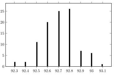
Figure 9

Histogram with the results obtained with 100 different initializations. Thex-axis plots the unlabeled attachment score on the test set, and they-axis plots the number of times a result occurred.

Effect of Initialization.The parser uses random seeds to create the mini-batches that it uses to train the model, which has an effect on the parsing results. In order to see the effect of initialization, we trained the whole S-LSTM parser with POS tags, pretrained word em-beddings, and composition functions on the English SD data set, for the same amount of time (around 20 hours) using different random seeds. Figure 9 shows the variation due to initialization for 100 different random seeds and their results on the English test set. We observe that even though the results are very similar with a minimum of 92.3 and a maximum of 93.1, there are differences. The modal result is 92.8.18

Effect of Beam Size. Beam search was determined to have minimal impact on scores (absolute improvements of ≤0.3% were observed with small beams). Therefore, all results we report used greedy decoding—Chen and Manning (2014) likewise only report results with greedy decoding. This finding is in line with previous work that generates sequences from recurrent networks (Grefenstette et al. 2014), although Vinyals et al. (2015),19 Zhou et al. (2015), and Weiss et al. (2015) did report much more substantial improvements with beam search on their parsers.

6.4 Experiments with Character-Based Word Representations

In order to isolate the improvements provided by the LSTM encodings of characters described in Section 4.2, we run the stack LSTM parser in the following configurations:

r

r

as in Section 4.2 (but without POS tags)

r

18 The results shown in Table 1 for the whole S-LSTM parser and English-SD are the best results for the development set, even though the histogram in Figure 9 shows a couple of models with better results on the test set.

r

LSTMs plus POS tags (Section 4.2)

r

(Section 4.1)

r

bidirectional LSTMs plus POS tags and morphological tags (Section 4.2)

None of the experimental configurations include pretrained word-embeddings or any additional data resources. All experiments includeSWAPtransition, meaning that nonprojective trees could be produced in any language. Finally, in addition to the dimensionality described in Section 6.1, the character-based representations of words have 100 dimensions.

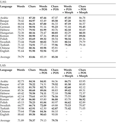
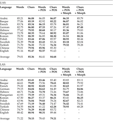
6.4.1 Results and Discussion. Tables 2 and 3 show the results of the parsers for the development sets and the final test sets, respectively. Most notable are improvements for agglutinative languages—Basque, Hungarian, Korean, and Turkish—both when POS tags are included and when they are not. Consistently, across all languages, Chars outperformsWords, suggesting that the character-level LSTMs are learning represen-tations that capture similar information to parts of speech. On average,Charsis on par withWords + POS, and the best average of labeled attachment scores is achieved with Chars + POS.

Even if our character-based representations are capable of encoding the same kind of information, existing POS tags suffice for high accuracy. However, the POS tags in treebanks for morphologically rich languages do not seem to be enough. This is evidenced by the results including explicit morphological features, which outperforms the ones without them in most cases, and outperforms the results using character-based representations. It is interesting to see that for some languages, such as German, Hungarian, Korean, and Swedish, the character-based representations seem to be enough to approach or even surpass the results of the parser by using rich morphologi-cal features. In Korean,Charsis the best model, which suggests that the character-based word representations encode as much useful information for parsing for that particular language as is currently available.

Swedish, English, and French use suffixes for the verb tenses and number,20 and Hebrew uses a root-and-pattern system. Even for Chinese, which is not morphologically rich,Charsshows a benefit overWords, perhaps by capturing regularities in syllable structure within words.

6.4.2 Out-of-Vocabulary Words.The character-based representation for words is notably beneficial for OOV words. We tested this specifically by comparingCharsto a model in which all OOVs are replaced by the string “UNK” during parsing. This always has a negative effect on LAS (average−4.5 points,−2.8 UAS). Figure 10 shows how this drop varies with the development OOV rate across treebanks; the most extreme is Korean, which drops 15.5 LAS. A similar, but less pronounced, pattern was observed for models that include POS.

Table 2

Unlabeled attachment scores (top) and labeled attachment scores (bottom) on thedevelopment

sets (not a standard development set for Turkish). In each table, the first two columns show the results of the parser with word lookup (Words) vs. character-based (Chars) representations. Boldface shows the better result comparingWordsvs.Chars, comparingWords + POSvs.Chars + POS, and comparingWords + POS + Morphvs.Chars + POS + Morph.

UAS:

Language Words Chars Words Chars Words Chars

+ POS + POS + POS + POS

+ Morph + Morph

Arabic 86.14 87.20 87.44 87.07 87.35 86.78

Basque 78.42 84.97 83.49 85.58 87.20 86.90

French 84.84 86.21 87.00 86.33 87.19 86.57

German 88.14 90.94 91.16 91.23 91.44 91.45

Hebrew 79.73 79.92 81.99 80.76 82.10 80.69

Hungarian 72.38 80.16 78.47 80.85 80.29 80.55

Korean 78.98 88.98 87.36 89.14 87.48 89.04

Polish 73.29 85.69 89.32 88.54 90.34 89.36

Swedish 73.44 75.03 80.02 78.85 80.14 79.79

Turkish 71.10 74.91 77.13 77.96 79.28 79.18

Chinese 79.43 80.36 85.98 85.81 – –

English 91.64 91.98 92.94 92.49 – –

Average 79.79 83.86 85.19 85.38 – –

LAS:

Language Words Chars Words Chars Words Chars

+ POS + POS + POS + POS

+ Morph + Morph

Arabic 82.73 84.34 84.81 84.36 84.71 83.95

Basque 67.08 78.22 74.31 79.52 81.50 80.85

French 80.32 81.70 82.71 81.51 82.68 82.12

German 85.36 88.68 89.04 88.83 89.42 89.31

Hebrew 69.42 70.58 74.11 72.18 73.98 72.37

Hungarian 62.14 75.61 69.50 76.16 75.55 75.85

Korean 67.48 86.80 83.80 86.88 83.78 86.92

Polish 65.13 78.23 81.84 80.97 84.62 82.89

Swedish 64.77 66.74 72.09 69.88 73.13 70.87

Turkish 53.98 62.91 62.30 62.87 71.42 71.05

Chinese 75.64 77.06 84.36 84.10 – –

English 88.60 89.58 90.63 90.08 – –

Average 71.89 78.37 79.13 79.78 – –

Interestingly, this artificially impoverished model is still consistently better than Words for all languages (e.g., for Korean, by 4 LAS). This implies that not all of the improvement is due to OOV words; statistical sharing across orthographically close words is beneficial as well.

Table 3

Unlabeled attachment scores (top) and labeled attachment scores (bottom) on thetestsets. In each table, the first two columns show the results of the parser with word lookup (Words) vs. character-based (Chars) representations. Boldface shows the better result comparingWordsvs.Chars, comparingWords + POSvs.Chars + POS, and comparing

Words + POS + Morphvs.Chars + POS + Morph.

UAS:

Language Words Chars Words Chars Words Chars

+ POS + POS + POS + POS

+ Morph + Morph

Arabic 85.21 86.08 86.05 86.07 86.35 85.79

Basque 77.06 85.19 82.92 85.22 86.87 86.02

French 83.74 85.34 86.15 85.78 86.81 86.21

German 82.75 86.80 87.33 87.26 87.40 87.48

Hebrew 77.62 79.93 80.68 80.17 81.36 79.83

Hungarian 72.78 80.35 78.64 80.92 81.07 81.06

Korean 78.70 88.39 86.85 88.30 86.84 88.24

Polish 72.01 83.44 87.06 85.97 88.93 88.44

Swedish 76.39 79.18 83.43 83.24 83.18 82.04

Turkish 71.70 76.32 75.32 76.34 79.52 78.28

Chinese 79.01 79.94 85.96 85.30 – –

English 91.16 91.47 92.57 91.63 – –

Average 79.01 85.36 84.41 84.68 – –

LAS:

Language Words Chars Words Chars Words Chars

+ POS + POS + POS + POS

+ Morph + Morph

Arabic 82.05 83.41 83.46 83.40 83.83 83.11

Basque 66.61 79.09 73.56 78.61 80.83 79.92

French 79.22 80.92 82.03 81.08 82.65 81.97

German 79.15 84.04 84.62 84.49 84.79 84.86

Hebrew 68.71 71.26 72.70 72.26 73.67 72.06

Hungarian 61.93 75.19 69.31 76.34 76.66 76.45

Korean 67.50 86.27 83.37 86.21 83.41 86.25

Polish 63.96 76.84 79.83 78.24 82.67 82.21

Swedish 67.69 71.19 76.40 74.47 76.42 74.41

Turkish 54.55 64.34 61.22 62.28 70.93 68.28

Chinese 74.79 76.29 84.40 83.72 – –

English 88.42 88.94 90.31 89.44 – –

Average 71.22 78.15 78.43 79.21 – –

0.05 0.10 0.15 0.20 0.25 0.30

−15

−10

−5

0

OOV rate

LAS dif

ference

zh enar

eu fr

de he

hu

ko pl sv

tr

Figure 10

On thex-axis is the OOV rate in development data, by treebank; on they-axis is the difference in development-set LAS betweenCharsmodel as described in Section 4.2 and one in which all OOV words are given a single representation.

Table 4

Unlabeled attachment scores and labeled attachment scores on thedevelopmentsets (top) and the finaltestsets (bottom) for Chinese and English (SD). The columns marked withWordsshow the results of the parser with the whole S-LSTM model presented in Section 6.3, and the column marked withWords + POSalso includes part-of-speech tags. The columns marked withWords + Charsshow the results of the parser when combining the pretrained word embeddings of Section 6.3 with the character-based representations of this section and the columns marked with

Words + Chars + POSalso includes part-of-speech tags.

Development:

Words Words + POS Words + Chars Words + Chars + POS

Language UAS LAS UAS LAS UAS LAS UAS LAS

Chinese 82.65 79.84 87.23 85.87 82.20 79.26 86.93 85.51

English 92.58 89.96 93.11 90.80 92.74 90.35 92.87 90.49

Test:

Words Words + POS Words + Chars Words + Chars + POS

Language UAS LAS UAS LAS UAS LAS UAS LAS

Chinese 82.15 79.04 86.85 85.36 81.90 78.81 86.92 85.49

English 92.57 90.21 93.04 90.87 92.56 90.38 92.75 90.62

6.4.3 Comparison with State-of-the-Art Parsers.Table 5 shows a comparison with state-of-the-art parsers. We include greedy transition-based parsers that, like ours, do not apply beam search. For all the SPMRL languages we show the results of Ballesteros (2013), who reported results after carrying out a careful automatic morphological feature selection experiment. For Turkish, we show the results of Nivre et al. (2006), who also carried out a careful manual morphological feature selection. Our parser outperforms these in most cases. For English and Chinese, we report our results of the best parser on the develpment set in Section 6.3—which isWords + POSbut with pretrained word embeddings.

Table 5

Test-set performance of our best results (according to UAS or LAS, whichever has the larger difference), compared with state-of-the-art greedy transition-based parsers (“Best Greedy Result”) and best results reported (“Best Published Result”). Note that B+’13 and B+’14 are a combination of parsers and use unlabeled data; our models do not. We only use unlabeled data for the pretrained word embeddings ofDWPP.Wrefers toWords;Crefers toChars;WPrefers toWords + Pos;WPMrefers toWords + Pos + Morph;CPrefers toChars + Pos;CPMrefers to

Chars + Pos + Morph; B’13 is (Ballesteros 2013); N+’06a is (Nivre et al. 2006);DWPPis our modelWord + Poswith pretrained embeddings and dynamic oracles as in Section 6.5;WPMis our modelWord + Pos + Morph; B+’13 is (Bj ¨orkelund et al. 2013); B+’14 is (Bj ¨orkelund et al. 2014); W+’15 is (Weiss et al. 2015).

This Work Best Greedy Result Best Published Result

Language UAS LAS System UAS LAS System UAS LAS System

Arabic 86.35 83.83 WPM 84.57 81.90 B’13 88.32 86.21 B+’13

Basque 86.87 80.63 WPM 84.33 78.58 B’13 89.96 85.70 B+’14

French 86.81 82.65 WPM 83.35 77.98 B’13 89.02 85.66 B+’14

German 87.48 84.86 CPM 85.38 82.75 B’13 91.64 89.65 B+’13

Hebrew 81.36 73.57 WPM 79.89 73.01 B’13 87.41 81.65 B+’14

Hungarian 81.07 76.66 WPM 83.71 79.63 B’13 89.81 86.13 B+’13

Korean 88.39 86.27 C 85.72 82.06 B’13 89.10 87.27 B+’14

Polish 88.93 79.83 WPM 85.80 79.89 B’13 91.75 87.07 B+’13

Swedish 83.43 76.40 WP 83.20 75.82 B’13 88.48 82.75 B+’14

Turkish 79.52 70.93 WPM 75.82 65.68 N+’06a 79.52 70.93 WPM

Chinese 85.96 84.40 WP 87.65 86.21 DWPP 87.65 86.21 DWPP

English 92.57 90.31 WP 93.56 91.42 DWPP 94.08 92.19 W+’15

set. For English, we report Weiss et al. (2015), and for Chinese, we report our results in Section 6.3—which isWords + POSbut with pretrained word embeddings and dynamic oracles (see next section).

6.5 Experiments with Dynamic Oracles

Table 6 shows the results of the parser with arc-hybrid and dynamic oracles for the English data set (with Stanford dependencies) and the Chinese CTB data sets with and without pretrained word embeddings, respectively. The table also shows the best result reported in Section 6.3 for the sake of comparison between static and dynamic training strategies.

The results achieved by the dynamic oracle for English are actually one of the best results ever reported in this data set, achieving 93.56 unlabeled attachment score. This is remarkable given that the parser uses a completely greedy inference procedure. Moreover, the Chinese numbers establish the state-of-the-art by using the same settings as in Chen and Manning (2014).

Table 6

Unlabeled attachment scores and labeled attachment scores on thedevelopmentsets (top) and the finaltest sets(bottom) for Chinese and English (SD). The columns marked with “Arc-std.” show the results of the parser arc-standard oracle, which are the same numbers as in Table 1. The columns marked with “Arc-hybrid” show the results of the parser with the arc-hybrid oracle. The columns marked with “static” (“dynamic”) show the results of the parser with static (dynamic) oracles.

Development

Arc-std. Arc-hybrid Arc-hybrid Arc-hybrid

(static) (static) (dynamic) (dynamic,α=0.75)

Language UAS LAS UAS LAS UAS LAS UAS LAS

Chinese (–pretraining) 85.96 84.37 82.65 79.84 85.96 84.37 86.32 84.59

Chinese (+pretraining) 87.23 85.87 87.11 85.64 87.41 85.99 87.41 85.87

English (–pretraining) 92.58 90.24 92.64 90.26 93.01 90.68 93.04 90.64

English (+pretraining) 93.11 90.80 93.16 90.88 93.38 91.03 93.51 91.29

Test

Arc-std. Arc-hybrid Arc-hybrid Arc-hybrid

(static) (static) (dynamic) (dynamic,α=0.75)

Language UAS LAS UAS LAS UAS LAS UAS LAS

Chinese (–pretraining) 85.48 83.94 85.66 84.03 86.07 84.46 86.13 84.53

Chinese (+pretraining) 86.85 85.36 86.94 85.46 87.05 85.63 87.65 86.21

English (–pretraining) 92.40 90.04 92.08 89.80 92.66 90.43 92.73 90.60

English (+pretraining) 93.04 90.87 92.78 90.67 93.15 91.05 93.56 91.42

6.6 Experiments with CoNLL 2009 Data Sets

In order to be able to compare with similar greedy parsers (Yazdani and Henderson 2015; Andor et al. 2016)21we report the performance of the parser on the multilingual treebanks of the CoNLL 2009 Shared Task (Hajiˇc et al. 2009). Because some of the treebanks contain nonprojective sentences and arc-hybrid does not allow nonprojective trees, we use the pseudo-projective approach (Nivre and Nilsson 2005). For all the experiments presented in this section we used the predicted part-of-speech tags pro-vided by the CoNLL 2009 shared task organizers. In order to see if the pretrained word embeddings are useful for other languages we also include results with pretrained word embeddings for English, Chinese, German, and Spanish following the same training set-up as in Section 4; for English and Chinese we used the same pretrained word embeddings as in previous experiments, for German we pretrained embeddings using the monolingual training data from the WMT 2015 data set22, and for Spanish we used the Spanish Gigaword version 3.

The results for the parser with character-based representations on these data sets (last line of the table) were published by Andor et al. (2016). In Zhang and Weiss (2016), it is also possible to find results of the same version of the parser on the Universal Dependency treebanks (Nivre et al. 2015).

21 We report the performance of these parsers in the most comparable set-up, that is, with beam = 1 or greedy.

Table 7

Results of the parser in its different versions including comparison with other systems. St. refers to static oracle with the arc-standard parser and Dyn. refers to dynamic oracle with the arc-hybrid parser withα=0.75 because it is the top scoring system in Section 6.5. PP refers to pseudo-projective parsing, SW refers to the arc-standard algorithm including the SWAP action as described in Section 3.3.2. +pre refers to the models that incorporate pretrained word embeddings. The Chinese treebank is fully projective and this is why we do not report results with SWAP since they are equivalent to the ones with pseudo-projective parsing. Y’15 is the parser by Yazdani and Henderson (2015). A’16 is the parser with beam = 1 by Andor et al. (2016). A’16-b is the parser with beam larger than 1 by Andor et al. (2016).Boldnumbers indicate the best results among the greedy parsers.

Catalan Chinese Czech English German Japanese Spanish

Method UAS LAS UAS LAS UAS LAS UAS LAS UAS LAS UAS LAS UAS LAS

St + PP 89.60 85.45 79.68 75.08 77.96 71.06 91.12 88.69 88.09 85.24 93.10 92.28 89.08 85.03

+ pre – – 82.45 78.55 – – 91.59 89.15 88.56 86.15 – – 90.76 87.48

St + SW 89.55 85.35 – – 78.66 71.99 91.12 88.50 88.11 85.48 93.29 92.46 89.02 84.96

+ pre – – – – – – 91.53 89.14 89.21 86.96 – – 90.43 86.99

Dyn + PP 90.45 86.38 80.74 76.52 85.68 79.38 91.62 89.23 89.80 87.29 93.47 92.70 89.53 85.69

+ pre – – 83.54 79.66 – – 92.22 89.87 90.34 88.17 – – 91.09 87.95

Y’15 – – – – 85.2 77.5 90.13 87.26 89.6 86.0 – – 88.3 85.4

A’16 91.24 88.21 81.29 77.29 85.78 80.63 91.44 89.29 89.12 86.95 93.71 92.85 91.01 88.14

A’16-b 92.67 89.83 84.72 80.85 88.94 84.56 93.22 91.23 90.91 89.15 93.65 92.84 92.62 89.95

Our parsers outperform the model by Yazdani and Henderson (2015). When com-paring with Andor et al. (2016), it is worth noting that they use pretrained word embeddings, plus predicted morphological features, and the top-KPOS tags from a CRF tagger instead of a simple predicted tags, so the results that are actually comparable are the ones in which we include pretrained word embeddings; our model is better than Andor et al. (2016), especially in the case of the dynamic oracles.

The results with Czech and the dynamic oracle model suggest that it is a much better strategy when the number of nonprojective trees is high; this result suggests that the training with exploration allows the parser to handle more complicated syntactic structures. Finally, the arc-standard parser enriched with the SWAP action performs similarly to the pseudo-projective approach for all languages, which demonstrates the effectiveness of both approaches when parsing nonprojective structures.

7. Related Work

Our approach ties together several strands of previous work. First, several kinds of stack memories have been proposed to augment neural architectures. Das, Giles, and Sun (1992) proposed a neural network with an external stack memory based on recurrent neural networks. In contrast to our model, in which the entire contents of the stack are summarized in a single value, in their model the network could only see the contents of the top of the stack. Mikkulainen (1996) proposed an architecture with a stack that had a summary feature, although the stack control was learned as a latent variable.

manually crafted and sensitive to only certain properties of the state, with the exception of Titov and Henderson (2007b), whereas we are conditioning on the global state. Like us, Stenetorp (2013) used recursively composed representations of the tree fragments (a head and its dependents). Titov and Henderson (2007b) used a generative latent variable based on incremental sigmoid belief networks to likewise condition on the global state. Neural networks have also been used to learn representations for use in phrase-structure parsing (Henderson 2003, 2004; Titov and Henderson 2007a; Socher et al. 2013; Le and Zuidema 2014). The work by Watanabe et al. (2015) is also similar to the work pre