Physician Income Prediction Errors: Sources and Implications for Behavior

PHYSICIAN INCOME PREDICTION ERRORS: SOURCES AND IMPLICATIONS FOR BEHAVIOR

Sean Nicholson Nicholas S. Souleles

Working Paper 8907

http://www.nber.org/papers/w8907

NATIONAL BUREAU OF ECONOMIC RESEARCH 1050 Massachusetts Avenue

Cambridge, MA 02138 April 2002

The University of Pennsylvania Research Foundation, Jefferson Medical College, and the Rodney L. White Center for Financial Research generously provided funding for the follow-up surveys. We are very grateful to Joseph S. Gonnella, Jon Veloski, Mary Robeson and other members of the Center for Research in Medical Education and Health Care at Jefferson Medical College for providing access to and assistance with the Jefferson Longitudinal Study. Patricia Danzon, Mark Pauly, Rob Lemke, Dan Polsky, and members of the macro lunch and the applied economics workshop at The Wharton School provided helpful suggestions, as did members of workshops at Stanford University, the University of Chicago, and the University of California-Berkeley, and participants at the Michigan/HRS/BLS Conference on Survey Research on Household Expectations and Preferences. Our research assistants provided valuable contributions: Josh Beer, Matt Cinque, Hanli Mangun, and Peter Margetis. The views expressed herein are those of the authors and not necessarily those of the National Bureau of Economic Research.

© 2002 by Sean Nicholson and Nicholas S. Souleles. All rights reserved. Short sections of text, not to exceed two paragraphs, may be quoted without explicit permission provided that full credit, including © notice, is given to the source.

Sean Nicholson and Nicholas S. Souleles NBER Working Paper No. 8907

April 2002

JEL No. J24, J3, J44, I11, D84

ABSTRACT

Although income expectations play a central role in many economic decisions, little is known about the sources of income prediction errors and how agents respond to income shocks. This paper uses a unique panel data set to examine the accuracy of physicians’ income expectations, the sources of income prediction errors, and the effect of income prediction errors on physician behavior. The data set contains direct survey measures of income expectations for medical students who graduated between 1970 and 1998, their corresponding income realizations, and a rich summary of the shocks hitting their medical practices. We find that income prediction errors were positive on average over the sample period, but varied significantly over time and cross-sectionally. We trace these results to persistent specialty-specific shocks, such as the growth of health maintenance organizations (HMOs) and other changes across health care markets. Physicians who experienced negative income shocks were more likely to respond by increasing their hours worked, allocating fewer of their work hours to teaching/research and more to patient care, and were more likely to switch specialties.

Sean Nicholson Nicholas S. Souleles

Health Care Systems Department Finance Department

The Wharton School The Wharton School

3641 Locust Walk 3641 Locust Walk

Philadelphia, PA 19104 Philadelphia, PA 19104

[email protected] and NBER

Tel: 215-898-9403 Fax: 215-573-2157

Income expectations are an important determinant of many economic decisions, including schooling and occupational choice. However, little is known about the accuracy of income expectations, the sources of income prediction errors, and how people respond to income shocks (Manski, 1993). Since income expectations are rarely directly observed, the most common approach in empirical applications is to assume that expectations are rational and infer income expectations from panel data on realized income. (See Dominitz and Manski (1997) for a review of this literature, and Willis and Rosen (1979) for an example of this approach.) However, Manski (1993) has shown that misspecifying how income expectations are formed can lead to incorrect inferences about peoples’ behavior given their expectations, for instance the responsiveness of school enrollment to the expected return to schooling.

There are only a few existing studies that assess the accuracy of income expectations, usually by comparing survey measures of income expectations with subsequent income realizations. Das and van Soest (1999) examine data from the Dutch Socio-Economic Panel, which asked people to predict whether in the next year their household income would decrease, remain unchanged, or increase. They find that between 1984 and 1989 their sample substantially underestimated their income growth; income

expectations were too pessimistic on average. Using a U.S. sample, Dominitz (1998) compares one-year-ahead income predictions in 1993, elicited in the form of subjective probabilities, with peoples’ actual income in 1994. He finds income expectations were too optimistic, by contrast.1

There are a number of limitations to the existing literature. First, one should not necessarily

1

Most other studies of the accuracy of household expectations have used aggregated data on inflation expectations (e.g.,Maddala, Fishe, and Lahiri, 1981; Gramlich, 1983; Batchelor, 1986). However, when agents’ information sets differ, aggregation can lead to spurious rejections of rationality. Some papers have indirectly modeled occupational choice without observing peoples’ subjective income expectations. Zarkin (1985) examines whether prospective teachers incorporate forecastable demand conditions into their decision to enter the occupation. He finds that future student enrollment rationally affects the occupational decisions of secondary school teachers, but not of elementary school teachers. Siow (1984) assumes that prospective lawyers expect future cohorts of students to arbitrage away any rents that would otherwise occur from a wage shock. He finds evidence consistent with his model.

expect prediction errors to average out to zero over a relatively short sample period (Souleles, 2001; Keane and Runkle, 1998). As a result, expectations that are rational ex ante might not appear rational ex post. For instance, the respondents in the two studies above might by chance have received positive and negative income shocks, respectively, over their short sample periods. Analyses of the accuracy of income expectations therefore require long sample periods. Souleles (2001) examines 18 years of monthly data from the Michigan Survey of Consumer Attitudes and Behavior. This survey records household expectations and subsequent realizations for a number of variables, including household income and financial security, inflation, and aggregate economic activity. Souleles finds that even over a long sample period, expectations of most of these variables appear to be biased and inefficient, at least ex post. He traces these results in part to aggregate shocks, like the business cycle and changes in monetary policy regime, as well as group-level shocks (e.g., shocks that disproportionately hit low education workers).

A second limitation of the literature is that the answers to the expectations questions are usually constrained to be discrete (e.g., Will income increase, decrease, or stay the same?), which complicates the analysis. Third, the expectations are usually limited to a one-year horizon, whereas life-cycle decisions like occupational choice depend on longer-horizon expectations. A final limitation is that most studies that reject the rationality of expectations do not explain why they reject, or whether the shocks that caused the prediction errors significantly altered people’s subsequent behavior.

In this paper we examine the accuracy of physicians’ income expectations, the sources of income prediction errors, and the effect of income prediction errors on physician behavior. We test, for example, whether the income prediction errors of specialists are significantly related to the advent of managed care, and whether physicians change their hours worked if their income turns out to be different than expected. We use a unique panel data set that allows us to overcome many of the limitations of previous studies of income expectations. The Jefferson Longitudinal Database contains information on all medical students

who graduated from Jefferson Medical College, a large medical school in Philadelphia, since 1970. The data set contains direct survey measures of medical students’ subjective income expectations, the

students’ actual practice income at various points during their medical career, and a rich set of

demographic and ability measures. In the fourth year of medical school, Jefferson students have been asked to predict the following: the specialty in which they will practice, their income 5, 10, and 20 years after completing residency training (i.e., their income with 5, 10, and 20 years of post-residency

experience), peak career income, and characteristics of their medical practice. In 1998 we devised a follow-up survey asking the same Jefferson physicians to report their current income, their income realizations in the same years for which they had previously stated their expected income, and the actual characteristics of their practice. The physicians were also asked to identify market and practice changes that occurred throughout their career, and to distinguish changes that were anticipated and unanticipated as of the time they formed their expectations. These unique questions allow us to reconstruct the physicians’ information sets and identify shocks that might explain their prediction errors.

The Jefferson Survey is particularly well suited to analyze income expectations because it solicits open-ended (continuous) income expectations over a person’s lifecycle. By 1998, the Jefferson graduates had been practicing medicine for up to 25 years, a period that might be long enough to allow negative and positive shocks to average out to zero if expectations are unbiased. Moreover, the sample period includes almost 30 cohorts of physicians. By contrast, if we tracked only a few cohorts of medical students, say those who graduated before 1975, then a large permanent shock to the physician services market in the late 1970s might lead one to reject the rationality of expectations based on incomes realized in the 1980s and 1990s. Medical students who graduate in the 1980s and 1990s, however, should have incorporated this shock into their own income expectations.

In a previous paper, Nicholson and Souleles (2001), we analyzed the original Jefferson income expectations data to try to identify the information that students use when forming income expectations,

and to examine whether subjective income expectations can help explain students’ specialty choices. We found that medical students condition their expectations in part on the contemporaneous income of physicians practicing in the specialty they plan to enter, but not on a one-for-one basis. This suggests that expectations are not strictly myopic.2 In fact, we found evidence that expectations are partly forward-looking: after students entering a given specialty reported relatively high income expectations, physicians in that specialty subsequently tended to experience higher income growth relative to other specialties, as measured by aggregated physician income data from the American Medical Association (AMA). We also found that the subjective income expectations were more useful in predicting specialty choice than contemporaneous physician income. These results suggest that the subjective expectations variables are quite informative. However, without the actual physician-specific realizations of income and other data solicited in the 1998 follow-up survey, we were not able to assess formally the accuracy of the

expectations, explore the sources of prediction errors, nor examine the welfare implications of prediction errors.

This paper examines a number of aspects of physician income expectations and realizations. First, we compare a physician’s actual income to the income he expected when he was a fourth-year medical student to gauge the accuracy of income expectations, including their unbiasedness and

efficiency. Second, and more importantly, we analyze the sources of any systematic prediction errors. In particular, can the results be explained by ex post shocks to realized income? The richness of the data allows us to analyze many salient possible shocks. For example, are income prediction errors more negative for female physicians? Do medical students under or over estimate the returns to ability? More generally, we examine how prediction errors vary cross-sectionally and over time. This allows us to characterize the shocks that have hit physicians in different specialties at different points between 1970 and 1998. For instance, to what extent did changes in the structure of health insurance in a physician’s

2

market, such as the emergence of health maintenance organizations (HMOs), lead to income prediction errors? Third, we examine whether shocks that cause income prediction errors significantly altered physicians’ subsequent behavior. How much flexibility do physicians have to respond to shocks, and along what margins do they respond? For instance, do they adjust their hours worked? In light of the central role of income risk in many economic decisions, such an analysis of income shocks should be of independent and general interest.

We find that medical students made systematic income prediction errors, even over the long, 28-year sample period. We trace the errors in large part to persistent specialty-specific shocks.

Unanticipated market and practice changes, such as changes in demand for physician services and in payments from health insurers, help explain much of the cross-sectional variation in prediction errors across physicians. For example, specialist physicians (e.g., surgeons and obstetricians) practicing in markets with relatively high HMO enrollment earned substantially less than they expected relative to physicians in these same specialties practicing in markets with average levels of HMO enrollment. More generally, the results call into question the common assumption that aggregate shocks affect people uniformly. Empirical implementations of rational expectations (or forward-looking) models therefore need to account for richer systematic heterogeneity in prediction errors. We also find that income prediction errors help explain subsequent physician behavior. Physicians who experienced negative income shocks were more likely to respond by increasing their hours worked, allocating fewer of their work hours to teaching/research and more to patient care, and were more likely to switch specialties. These results imply that market and practice shocks have substantial welfare effects.

The rest of this paper is organized as follows. We describe the data in more detail in Section II. In Section III we present the empirical method for assessing the accuracy of income expectations, identifying the sources of income prediction errors, and examining the effect of prediction errors on

changes that physicians make to their medical practice. We present results in Section IV and offer concluding comments in Section V.

II. Data

The Jefferson Longitudinal Database contains unique information about physicians’ expectations regarding their medical practice. In 1970 Jefferson Medical College began surveying its medical students in their fourth year of medical school. Students are asked to predict the specialty in which they will practice and their income from medical practice. Between 1970 and 1979, students were asked to state the income, after medical expenses and before taxes, they expected to receive 5, 10, and 20 years after completing residency training, and the peak income they expected to receive during their career.3 Students were asked, “…(to) assume that dollars maintain their present value …” when stating their expected income. Students who graduated after 1979 have been asked to predict only their peak income, not income after 5, 10, and 20 years of experience. The Jefferson Longitudinal Study contains

information on all 5,995 alumni who graduated between 1970 and 1998, most of whom are now practicing physicians. In the first column of Table 1 we report means of key variables for the entire sample.

The Jefferson database includes demographic information and rich measures of student ability and performance in school. Medical students must pass three national exams before they can receive a license to practice medicine in the United States. Part 1 of the National Board of Medical Examiners (NBME) test is administered after the second year of medical school and covers the classroom material taught during the first two years (e.g., anatomy, physiology, pharmacology).4 Jefferson students who

3

Most medical students complete between three and five years of residency training, depending on the specialty, before practicing medicine. We consider a physician to begin “practicing medicine” when he completes residency training.

4

The second part of the NBME exam is administered in the fourth year of medical school and the third part is administered in the first year of a student’s residency program. We focus on the Part 1 score as a measure of student ability and performance because this exam occurred before students stated their income expectations.

graduated between 1996 and 1998 received an average score of 209.1 on Part 1 of the NBME, referred to hereafter as the board score. The average board score for all students who graduated from a U.S. medical school during this same time period was 210.8, so Jefferson students appear to be generally representative of U.S. medical students.5

In 1998 we mailed surveys to all the individuals who graduated from Jefferson Medical College between 1970 and 1979, the period during which students predicted their income with 5, 10, and 20 years of post-residency experience, as well as their peak career income. In 1998 these alumni had been

practicing medicine between 13 and 25 years. They were asked to report current characteristics of their practice such as their specialty, the average number of hours they work per week, and their patients’ sources of health insurance. The Jefferson alumni also reported their medical practice income (after expenses but before taxes) for the previous year (1997), as well as their practice income 5, 10, and 20 years after they completed residency training, without making any adjustments for inflation.6 These income realizations correspond in time to the income expectations the physicians provided when they were fourth-year medical students. An impressive 93 percent of the physicians who completed the 1998 follow-up survey reported their practice income for each year requested.

The follow-up survey allows us to calculate income prediction errors -- the difference between actual and expected income -- for each respondent in their 5th, 10th, and,for older physicians, their 20th year of practicing medicine. Since the income prediction errors, like other variables solicited from surveys, will inevitably be measured with some error, we also asked physicians the following question: “Overall, how did your actual practice income in your 10th year [or 20th year for older physicians] compare with the income that you expected when you were a fourth-year medical student (after taking

5

The standard deviation of the board score among students who graduated from U.S. medical schools between 1996 and 1998 is 18.

6

The question for 1997 income was worded as follows: “Please estimate your income from medical practice in 1997 to the nearest $10,000, after professional expenses but before taxes. Please include all income from fees, salaries, risk pools, retainers, bonuses and other forms of compensation.”

inflation into consideration)?” The physician could report that his actual income was higher, lower, or about the same as previously expected. This “subjective assessment” variable allows us to instrument for a respondent’s income prediction error when it is used as an independent variable in analyzing the impact of the errors on subsequent behavior. We undertake additional checks for measurement error below.

The 1998 follow-up survey tried to identify the reasons why a physician’s realized income might be higher or lower than had been expected. Physicians who have been practicing medicine for 20 years or more were asked to identify changes in the health care market (e.g., a decrease in the payments received from health insurance companies, or an increase in demand for their services) and changes they made to their practice (e.g., an increase in hours worked) that occurred during their first 20 years of practicing and had a significant effect on their income in the 20th year. Physicians who had been practicing for fewer than 20 years were asked a similar question regarding their experience during the first 10 years of practicing medicine. The physicians were then asked to indicate which of these market and practice changes had been expected when they were fourth-year medical students. This information allows us to reconstruct a student’s information set at the time he stated his expected income. Household data sets rarely contain such rich data regarding information sets.

In the 1998 follow-up survey we also asked physicians to identify any substantial changes they made to their practice (e.g., changes in hours worked, or in the number of uninsured patients treated)

since their 20th or 10th year of practicing medicine, depending on whether the respondent had been

practicing for more than or fewer than 20 years. This information allows us to examine whether and how physicians altered their behavior in response to shocks they faced over their careers, as measured by the income prediction errors. We also asked the Jefferson alumni to forecast their retirement age and whether, with hindsight, they would have selected the same specialty in medical school, selected a different specialty, or would have left the medical profession altogether.

Medical College between 1980 and 1998. After 1979 Jefferson asked its students to predict only their peak income. Therefore, the 1999 follow-up survey splits physicians into two groups according to their response to the following question: “Do you think that your income from medical practice has already peaked, or has not yet peaked.” Physicians who believed their income had already reached its maximum value, after taking inflation into consideration, were asked to report the year in which their real income from medical practice peaked as well as the actual peak amount. For these physicians we can calculate an income prediction error by comparing the actual peak income to the peak income expected as of the fourth year of medical school, with both variables adjusted for inflation.

Respondents who believed in 1999 that their income had yet to reach its peak were asked to report their current expectations for peak income. This allows us to calculate the difference between a respondent’s current expectation for peak income and his expectation for peak income when he was a fourth-year medical student. Like the prediction errors, this difference reflects the arrival of new information. All respondents of the 1999 follow-up survey were also asked to report their income from medical practice for the most recently completed year (1998), as well as their practice income for 1992. We structured the rest of the follow-up survey for the 1980-1998 graduates in the same way as the survey for the 1970-1979 graduates. Members of the former group were asked to document changes in the health care market and their practice between the year they graduated from medical school and either the year in which their income peaked, or 1999 if they believed their income had yet to reach its peak. They were asked to identify changes they made to their practice since their income peaked, or changes they expect to make in the future if they believe their income has not yet peaked. The students also provided subjective assessments of whether their actual peak income was higher, lower, or about the same as expected (or whether their current expectation for peak income was higher, lower, or about the same as their original expectation for peak income).

follow-up surveys. This is an unusually good response rate for a mail survey, especially in light of the sensitive nature of the income and other survey questions. Even so, since we know a great deal about the non-respondents from the survey and other information collected during medical school, we can check for evidence of selection bias in completing the follow-up survey. Means for the main variables collected during medical school are reported in column 2 of Table 1 for those individuals who completed the follow-up survey. In general, the characteristics of the respondents to the follow-up survey are quite similar to the entire population of students who graduated between 1970 and 1998 (column 1). Relative to the non-respondents, the respondents are slightly younger, are more likely to be male and white, have slightly higher board scores (ability), and were slightly more likely to become a family practitioner and less likely to become a radiologist.7 However, these differences are all small in magnitude, and the analysis below will control for these characteristics as well as the physicians’ own characterization of the shocks to their practices. Hence, any remaining unobserved heterogeneity is unlikely to systematically explain our results, especially the cross-sectional results that we highlight. Further, there is no

statistically significant difference in expected income between respondents and non-respondents, which suggests that respondents do not substantially differ in unobserved ability either. Overall, there is little evidence of systematic selection in the follow-up sample.

Table 2 reports means and standard deviations for the sample of 2,350 individuals who returned the follow-up survey and had completed their residency training at the time of the survey. This and subsequent tables exclude from the analysis the 281 respondents who were still residents and so not yet practicing. As reported in the middle of Table 2, about one-third (0.366) of the practicing respondents believe their actual income with 10 years of experience, 20 years of experience, or their peak income was higher than they expected when they were a fourth-year medical student, and a similar percentage believe it was lower than expected. Hence, there is substantial variation in the physicians’ subjective assessments

7

of the signs of their income prediction errors. About 20 percent of the respondents would have chosen a different specialty in medical school or left the medical profession entirely given what they have learned since graduation.

Turning to the bottom of Table 2, a fairly large proportion of physicians have experienced changes in their market or have made changes to their practice that had a significant effect on their income (or their expected peak income). Few of these physicians anticipated these changes when they were in medical school. The second column at the bottom of the table reports the proportion of those

experiencing a change that expected the change when they were in medical school. For example, 51

percent of the physicians report that demand for their services increased between the time they graduated from medical school and their 10th or 20th year of practicing, or the year in which their income peaked. However, only 35 percent of the physicians who experienced a demand increase anticipated this change when they were a fourth-year medical student. For most physicians, therefore, the increase in demand can be characterized as a shock – an unforeseen event that could affect income but not expected income. Similarly, most of the 57 percent of physicians whose payments from insurance companies decreased were surprised by this change. On the other hand, less than 10 percent of physicians report they significantly decreased their hours worked, but about one-third of them expected to do so.

In the last two decades managed care health plans, such as health maintenance organizations (HMOs) and preferred provider organizations (PPOs), have replaced fee-for-service plans as the dominant form of health insurance in the United States. We want to measure the extent to which this

transformation of the health insurance market represented a shock to physicians’ incomes. In 1976, less than three percent of the U.S. population was enrolled in an HMO.8 Relative to a traditional fee-for-service health plan, HMOs generally cover more health fee-for-services (e.g., pharmaceuticals and preventive care), require patients to pay relatively less when they receive medical care, and charge a lower premium.

HMOs are able to offer a more comprehensive product for a lower price by restricting enrollees’ choice of physicians and hospitals, negotiating lower fees with physicians and hospitals included in the network, and more aggressively managing the care that patients receive, for example by requiring patients to receive permission from their primary care physician before seeing a specialist. HMO enrollment has grown rapidly over the past two decades as individuals and businesses have sought to limit the growth rate of health spending. By 1999, about 30 percent of the population was enrolled in an HMO, and even more were enrolled in less restrictive managed care health plans such as PPOs.

Studies have shown that HMOs reduce their enrollees’ use of hospital services and negotiate lower payments to hospitals for these services (Miller and Luft, 1994; Cutler, McClellan, and Newhouse, 2000). The evidence is mixed regarding whether HMOs increase or decrease their enrollees’ use of physician office visits (Miller and Luft, 1994). Despite the widespread impression that HMOs have reduced physicians’ incomes, there has been little empirical evidence confirming this effect.9 Many of the students in our sample graduated when HMOs were uncommon. Suppose the Jefferson students did not expect HMOs, and managed care plans generally, to be as prevalent as they are. Then the physicians who located in areas that subsequently experienced considerable growth of HMO enrollment might earn much less than expected, ceteris paribus, especially in non-primary care specialties.

We use data from Interstudy, a research organization that studies managed care health plans, to determine the percentage of the population in each physician’s state that was enrolled in an HMO in each year. We know the state in which a respondent lived in 1998 or 1999, but do not know their residence in prior years. We assume, therefore, that a physician has practiced medicine in their current state

8

Based on data from Interstudy.

9

Simon et al. (1996) find that between 1985 and 1993 primary care physicians practicing in states with relatively high managed care enrollment experienced relatively large income increases, whereas the opposite was true for hospital-based physicians (radiologists, anesthesiologists, and pathologists). Thisresult is consistent with the widely held view that primary care physicians will fare better than non-primary care physicians in a market dominated by managed care health plans.

continuously since completing residency training.10

III. Empirical Method

We begin by formally testing whether medical students’ income expectations are unbiased and efficient. Income expectations are unbiased if the mean prediction error is zero. We compute the income prediction error of physician i in the jth year after completing residency training as the difference between realized income (Yi,j) and expected income (EYi,j,t=0). We test for unbiasedness by regressing this error on

a constant: . u + α = EY Y (1) i,j− i,j,t=0 0 1

We convert expected and realized income to 1996 dollars using the urban consumer price index (CPI), and we correct the standard errors to allow for correlation in the error terms between physicians who received income in the same year, which allows for common shocks. The income expectations were reported when the respondent was a fourth-year medical student (t=0), and actual income was reported retrospectively in the 1998 or 1999 follow-up survey. The mean prediction error (α0) could be non-zero

because of systematic shocks in the physician services market. In this case unbiasedness might be rejected ex post even if students make ex ante optimal forecasts given the information that was available to them. However, because our sample period is quite long, extending almost 30 years during which there should have been both positive and negative income shocks, the shocks should be more likely to average out than in previous studies of income expectations. In any case, our data will allow us to characterize the sources of systematic income prediction errors.

Income expectations are efficient if people use all of the information available to them to forecast their income. Time series analyses of efficiency often test for serial correlation in prediction errors.

10

Since some physicians move during their careers, our HMO enrollment variable will be measured with some error, which will tend to attenuate our estimates of its effects. Polsky et al. (2000) find that between 1.5 and 2.0 percent of physicians relocated their practice to another metropolitan area per year between 1988 and 1992.

However, our micro data set contains few income prediction errors per physician (two or three errors for physicians who graduated before 1980, and only one error for the physicians who graduated after 1980). Therefore to test efficiency this paper instead focuses on cross-sectional variation, and looks for

systematic demographic components in the prediction errors. Specifically, we add to the specification variables Xi in physician i's information set at the time of forecast (t=0), including personal

characteristics:

.

u

+

+

β

=

EY

-Y

(2)

β

X

If any of the β1 coefficients are non-zero, the efficiency hypothesis is rejected.

We further examine the sources of income prediction errors by adding variables Zi,j that might

have affected physician i’s income in year j, but were not necessarily in his information set in year zero:

u

+

=

EY

-Y

(3)

γ

T

+

γ

X

+

γ

Z

We include a full set of year dummies (T) to identify the timing of aggregate shocks to the market for physician services. Indicator variables for a physician’s specialty are included in Z to see whether

unexpected shocks had a different effect across specialties. Z also contains the percentage of the

population in physician i’s state that is enrolled in an HMO in year j. This measure of HMO penetration is sometimes interacted with the set of specialty indicators because HMOs might exert a different effect on different specialties. A common assumption is that by requiring patients to begin their treatment with a primary care physician (i.e., family practitioner, pediatrician, or a general internist) who then decides whether a specialist referral is necessary, HMOs would favor primary care relative to non-primary care

physicians.

We also include in Z the self-reported changes in a physician’s market, such as a decrease in the payments received from health insurance companies, and changes physicians made to their practices, such as decreasing the fraction of uninsured patients treated. If medical students anticipated these market and practice changes when they formed their income expectations, they should not be highly correlated with the income prediction errors. For each type of market or practice change, therefore, we include an indicator if the physician reported that the change occurred and was anticipated when the respondent was a fourth-year medical student, and a separate indicator if the change occurred but was not anticipated. Unexpected changes should be correlated more strongly with the income prediction errors than are expected changes.

The prediction errors are the difference between realized and expected income. It is sometimes informative to examine separately the determinants of realized income and of expected income. Since Nicholson and Souleles (2001) already analyzed the income expectations, we focus here on the income realizations. We regress realized income in year j on a set of indicators for the year in which income was received (T), personal characteristics (X), and characteristics of a physician’s market and practice (Z):

.

4

(

)

Y

=

δ

T

+

δ

X

+

δ

Z

+

u

Z includes the measure of HMO penetration and practice characteristics, such as the average number of

hours worked per week and the proportion of patients who are uninsured.

Finally, we examine whether physicians alter their behavior after shocks cause their actual income to be different than expected, or after shocks cause physicians to revise their income predictions. Let Pt represent a characteristic of physician i’s practice in year t, such as the number of hours worked per

Physicians were surveyed at time j + k (1998 or 1999) and asked to report changes they have made to their practice since year j, where j is either their 10th or 20th year of practicing medicine. The probability that a physician changes a characteristic of his practice between year j and j + k is assumed to be a function of his income prediction error in year j, Yi,j - EYi,j,t=0, controlling for his actual income in year j

and personal characteristics (X):

.

To maximize sample size, for physicians whose income has not yet peaked, the dependent variable is a change the physician expects to make in the future and the revision in expected peak income (EYpeak,t=1999

– EYpeak,t=0) is used instead of the prediction error.11 A non-zero coefficient for θ1 indicates that

physicians alter their behavior in response to unanticipated income shocks.

IV. Results

a. Income Prediction Errors

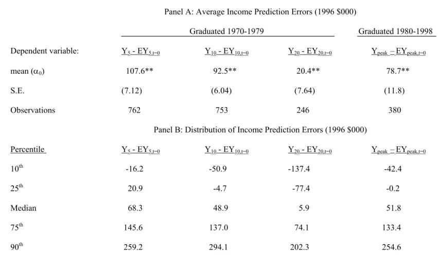
Table 3 reports the average prediction error, separately for 5, 10, and 20 years of experience, and for physicians’ peak income if they believe their income has already peaked. The income prediction errors for 5, 10, and 20 years of experience (columns 1-3) are from the students who graduated between 1970 and 1979, whereas the peak income prediction errors (column 4) are from the students who graduated between 1980 and 1998. For comparability we express all dollar values in 1996 dollars. We regress a person’s income prediction error for each experience level on a constant term as described in equation (1). The null hypothesis of unbiasedness is that the coefficient on the constant term (α0) is zero.

(P

(5) i,j+k −Pi,j) =

θ

θ

θ

11

Recall that for physicians who believe their income has not yet peaked, the follow-up survey asked them to identify changes they expect to make in the future, and to re-forecast their peak income. About 35 percent of the observations used in the results for equation (5) employ these revisions to peak income. The conclusions are

qualitatively the same, however, without these observations. The analyses of prediction errors using equations (1) to (3) do not use the revisions to expected peak income.

α0 is positive and significantly different from zero for all four experience levels. Income was on

average significantly greater than expected, especially early in physicians’ careers: α0 is $107,600 with 5

years of experience but considerably smaller ($20,400) with 20 years of experience. The result for peak income in the final column is generally consistent with the previous columns: the physicians reporting peak income had fewer than 16 years of experience at the time of the follow-up survey. Therefore, it appears that average income prediction errors generally decline with the forecast horizon.

The bottom panel of Table 3 presents the distribution of income prediction errors by years of experience. The median physician earned $68,300 more than he or she expected after five years of practicing medicine, $48,900 more than expected after 10 years, and $5,900 more than expected after 20 years of experience. The median income prediction error for physicians whose income has already peaked is $51,800. There is substantial heterogeneity in the income prediction errors. Although the mean prediction error is positive for all experience levels, a considerable number of physicians earned less than they expected after 10 and 20 years of experience. The difference between the 75th and 25th percentile of errors is about $120,000 for 5 and 10 years of experience, and almost $150,000 for 20 years of

experience. Thus, although the average prediction errors decline with the forecast horizon, the cross-sectional variance of the errors increases with horizon.

It is possible, of course, that measurement error affects these results. The larger errors at lower levels of experience could be due to recall bias that worsens with the horizon. For example, for some physicians the 5th year of experience occurred as many as 21 years before the follow-up survey. Suppose that a physician who is asked to recall his income at a relatively distant point in the past reports an amount that is biased toward his current income, which is generally larger than the income he is recalling. Such a bias could generate prediction errors that decrease with the forecast horizon. We test this

hypothesis by pooling the 5, 10, and 20-year prediction errors and regressing them on a constant, separate indicators for 5 years and 10 years of experience, and a variable measuring the number of years elapsed

between the year of income receipt and the follow-up survey. While the indicators for 5 and 10 years of experience remain significantly positive, with a larger coefficient for 5 years, the number of years elapsed is insignificant.12 Thus, the large prediction errors are associated with being in the 5th year and 10th year of experience per se, even if the 5th year and 10th year took place relatively recently. The prediction errors are not associated with the time elapsed, counter to the hypothesis of systematic recall bias.13

Further, the results are similar if we analyze the revision in expected peak income for physicians who believe their income has not yet peaked (EYpeak,t=1999 - EYpeak,t=0). Here the current expectation for

peak income from the follow-up survey is not subject to recall bias. The corresponding mean revision (α0) is 45.6 (standard error of 5.93), which implies that these physicians on average received good news,

and revised up their expectations for peak income. Furthermore, recall bias is unlikely to explain the systematic cross-sectional components of the prediction errors that we emphasize below. For instance, there is no reason to suppose that recall bias differentially affects female versus male physicians, or physicians in states with high HMO enrollment versus those in states with low HMO enrollment.

There are a number of other possible explanations for the result that the average prediction errors decrease with the forecast horizon. First, it could be that shocks to the health care market

disproportionately benefited younger physicians. To explain the results, however, successive cohorts of young physicians must have received positive shocks repeatedly over the sample period. As noted below, the average forecast error is positive for every cohort in the sample.14 Second, it could be that students are

12

The coefficient on the number of years elapsed is also insignificant if we also include in the regression prediction errors for physicians whose income has already peaked.

13

A related form of recall bias might involve money illusion. Suppose physicians underestimated the amount of inflation that occurred between the year of income receipt and the follow-up survey, for example in the late 1970s. They might then report too large a figure for nominal income for the early part of their careers. We test this hypothesis by regressing the pooled 5, 10, and 20-year prediction errors on a constant, indicators for 5 years and 10 years of experience, and the change in the CPI between the year of income receipt and the follow-up survey. The coefficient on the change in the CPI is insignificant.

14

Souleles (2001) notes that such a result is not unlikely when the relevant “regime” is long lasting. For instance, he finds that low education workers continued to receive disproportionately negative shocks over the 1980's and 1990's, perhaps due to ongoing and unexpected skill-biased technical change. As a result he concludes that it is very difficult to distinguish ex ante bias from ex post shocks. Similarly, here the shocks due to different

generally better at forecasting over long rather than short horizons. Since income shocks can be persistent, however, this seems unlikely. Note that the same students are forecasting over the different horizons, so one cannot conclude that students are uniformly pessimistic. Third, students might be relatively pessimistic regarding the beginnings of their careers. Anecdotes suggest that many medical students are not fully aware of how steeply income rises early in physicians’ careers, perhaps because students unduly extrapolate their low incomes during the lengthy period of medical training. Students might receive more accurate information regarding the income of very experienced physicians, perhaps because the clinical faculty who have a great deal of contact with third- and fourth-year medical students have considerable experience. We further analyze this explanation below.

To test for efficiency, we regress the income prediction errors on variables that were in students’ information sets when they stated their expected income, using equation (2). Results are reported in the first column of Table 4. The prediction errors for 5, 10, and 20 years of experience, and for peak income are pooled together, with experience and experience squared included as controls.15 Standard errors are adjusted to allow for correlation within an individual across different experience levels.

The estimated coefficients for experience are jointly significant. The prediction errors with 5 years and 10 years of experience are $87,000 and $76,000 larger, respectively, than the prediction errors for 20 years of experience, consistently with Table 3, even controlling for demographic characteristics.

The coefficient for female physicians is significantly negative. Nicholson and Souleles (2001) showed that females expected to earn less than men, controlling for a similar set of covariates. Evidently their incomes turned out ex post to be even lower than expected, to a substantial degree. The difference between realized and expected income was $56,700 lower, on average, for women relative to men. Hence the gender gap does in fact represent a large, negative shock to women. One explanation for this result

health care regimes can also be prolonged.

15

The results include the prediction errors for peak income for physicians whose incomes have peaked, but not the revisions to expectations of peak income for physicians whose incomes have not yet peaked. Consistently with Table 3, more than 80 percent of the observations are prediction errors for 5, 10, and 20 years of experience

that we will examine later is that women, particularly those with young children, work fewer hours than men, and women might underestimate the impact of childrearing on their income when forming income expectations. White physicians earned $35,000 more than they expected relative to non-white physicians, whereas the coefficient on ability (the board score) is not significantly different from zero.

The three physician-specific characteristics (female, white, board score) are jointly significant. While these results represent a formal rejection of efficiency, one cannot conclude that students

systematically differed in the ex ante quality of their income forecasts. Different types of students might have received different shocks ex post, even on average over the long sample period. Furthermore, these demographic characteristics and experience explain relatively little of the variation in income prediction errors between physicians; the R2 in the first column of Table 4 is only 0.04.

The remaining columns of Table 4 use equation (3) to further explore the sources of income prediction errors. The second column includes as independent variables only experience and a full set of dummies for the year in which a physician received his income. The time dummies control for aggregate shocks that (uniformly) affected all physicians. The year indicator variables are jointly significant. Thus, the average prediction errors vary significantly over time. As will be discussed below, the largest income prediction errors occurred in the late 1980s, although on average the students earned more than they expected in every year. Nonetheless, aggregate shocks explain relatively little of the variation in income prediction errors; the R2 in the second column is only 0.04.

The third column of Table 4 focuses instead on additional cross-sectional heterogeneity in prediction errors. In light of the large differences in income between specialties, we replace the year dummies with specialty indicator variables. Although the Jefferson alumni have generally earned more than they expected, there are substantial differences by specialty. Students who entered internal medicine sub-specialties (e.g., cardiology or gastroenterology), radiology, anesthesiology, and surgery earned over

$100,000 per year more than they expected, relative to students who entered family practice (the omitted specialty), on average. Under the assumption that the ex ante quality of students’ forecasts do not vary across specialties, this suggests that different specialties received different income shocks ex post. That is, there are specialty-specific shocks that the aggregate time dummies cannot soak up. The R2 of 0.16 indicates that specialty-specific shocks alone explain a considerable amount of the variation across physicians in income prediction errors, more than year dummies and personal characteristics.

An alternative interpretation of the difference in errors across specialties is that medical students are not particularly knowledgeable about physician income, and the quality of their knowledge varies across specialties. However, this assessment is not consistent with the analysis by Nicholson and Souleles (2001). They find that students do in part foresee future relative trends in specialty income and incorporate these changes into their own expectations, although not on a dollar for dollar basis. That is, while their expectations are sensitive to future income trends, some of these trends are unexpected.

Further, if the average specialty errors simply reflected differential knowledge across specialties, one might expect the relative errors to be rather constant over time. However the relative errors change over time. This again suggests that different specialties received different shocks over time. To illustrate this result, we group the specialties into two categories: non-primary care physicians (surgeons,

radiologists, internal medicine sub-specialists, obstetricians, pathologists, psychiatrists, and

anesthesiologists) and primary care physicians (family practitioners, internists, and pediatricians). We then interact the year indicators (as in the second column of Table 4) with an indicator that equals one for the non-primary care physicians. The interaction terms are jointly significant and their inclusion

increases the R2 from 0.04 in column 2 to 0.09 (not reported).

In Figure 1 we plot the mean income prediction error over time, separately for primary and non-primary care physicians. To increase precision, the time dummies refer to two-year increments.16 For

16

primary care physicians the mean income prediction error is always positive, and significantly different from zero at the five-percent level for every time period. Relative to primary care physicians, non-primary care physicians’ income was much larger than expected, especially so in the late 1980s.17

The gap between the lines in Figure 1 characterizes the relative shock to non-primary care versus primary care physicians. Even if recall bias or other measurement issues affect the overall sample average prediction error, they are unlikely to explain the fluctuations in this gap. The fluctuations in relative errors are indicative of time-varying, specialty-specific shocks. The relative positive shock to non-primary care income in the 1980s might be due in part to new medical technologies (e.g., MRI, arthroscopic surgery, laparascopic surgery, and angioplasty) that increased the demand for specialist services.18 The relative negative shock to non-primary care physicians that occurred in the early 1990s could be due to the influence of managed care health plans on the physician services market and the 1992 revision to the Medicare fee schedule that favored primary care physicians. We will further examine these shocks below.

These results have important methodological implications for rational expectations (or forward-looking) models. Empirical implementations of such models usually rely on time dummies to soak up all systematic components of prediction errors, assuming that aggregate shocks hit all people uniformly.19 However, our results suggest that time-varying, group-specific shocks, which are not captured by time dummies, are also important. Empirical models need to account for such systematic heterogeneity in prediction errors.

The final column of Table 4 includes year indicators, specialty indicators, and personal

17

The non-primary care - year interactions are always positive, and significant at at least the 10-percent level for every 2-year bin in the sample period.

18

Because of entry barriers in the non-primary care specialties, these technology shocks were not fully offset by more residents switching into non-primary care. Many medical students who tried to obtain residency positions in orthopedic surgery, surgery, radiology, and obstetrics in the 1980s were unsuccessful (Nicholson, 2001).

19

In many empirical specifications the prediction errors are relegated to the residual term and assumed to be classical. However, if the prediction errors are systematic (e.g., they are correlated with basic demographic

characteristics. These variables collectively explain 19 percent of the variation in income prediction errors. This R2 is large considering that classical income prediction errors should be white noise. Evidently prediction errors are not as classical as usually assumed. Controlling for specialty and year, women still earned less than they expected relative to men, as did non-whites.

b. Income Realizations

Nicholson and Souleles (2001) already analyzed one component of the income prediction errors, the income expectations. Here we analyze the other component -- the income realizations elicited in the follow-up surveys. Although there are up to four separate income observations for each respondent, information on the characteristics of their practice is available only for the time of the follow-up survey, either in 1998 or 1999.20 We therefore perform two separate regressions, both following equation (4). First, we pool the multiple income observations for each respondent and regress them on personal characteristics, including experience, market characteristics (e.g., HMO penetration over time), and specialty indicators. In this specification the standard errors are adjusted to allow for correlation in the error terms between the multiple observations for an individual. HMO penetration is interacted with the specialty indicators to allow the effects of HMOs to vary across specialties. Second, we regress a physician’s income in 1997 or 1998 on personal characteristics, specialty indicators, as well as contemporaneous practice characteristics (in 1998 or 1999).

The results of the first regression with multiple income observations over physicians’ careers are reported in the first column of Table 5. Controlling for specialty and ability, as measured by the board

See Souleles (2001) for a discussion.

20

Recall that the first follow-up survey (in 1998) was sent to students who graduated from medical school between 1970 and 1979. Among this group, physicians who had been practicing medicine for fewer than 20 years were asked their income with 5 years of experience, 10 years of experience, and for 1997 (the most current complete year at the time of the survey). Physicians who had been practicing medicine for 20 or more years were also asked their income with 20 years of experience. The second follow-up survey (in 1999) was sent to students who graduated between 1980 and 1998. These physicians were asked to report their income in 1998 (the most current complete year), 1992, and their peak income if they believed their income had already peaked.

score, women earned $59,600 less, on average, than men. The estimated coefficients for experience and experience squared, which are jointly significant, imply that annual practice income increased by $43,000 (in real dollars) in the first five years of a physician’s career, increased by $24,000 between the fifth and 10th year of experience, and decreased by $9,000 between the 10th and 20th years of experience. That is, the experience-income profile is quite steep at low levels of experience and peaks before 20 years of experience. As suggested above, medical students might not be fully aware of the initial steepness of the experience-income profile.

The uninteracted variable for HMO penetration, corresponding to family practice, is insignificant. The HMO-specialty interactions, however, are statistically significant for several non-primary care specialties.21 Relative to family practice, specialists in fields like internal medicine sub-specialties, surgery, ob/gyn, and anesthesiology in states with high levels of HMO activity earn significantly less than comparable physicians practicing in those specialties in states where HMOs are less prominent. These effects are also economically significant. For example, a cardiologist in a state where 20.9 percent of the population is enrolled in an HMO (the mean value for the physicians in the sample) is predicted to earn $33,400 less per year than an otherwise similar cardiologist practicing in a state where only 11.2 percent of the population is enrolled in an HMO (one standard deviation lower than the mean).

HMO enrollment has grown rapidly in the United States, especially between 1992 and 1998 when enrollment grew at an average rate of 12.4 percent per year. The growth of HMOs could constitute the negative shock experienced by non-primary care physicians relative to primary care physicians in the 1990s that is illustrated in Figure 1. After 1993 the relative income prediction errors for non-primary care physicians relative to primary care physicians began to decline.

The second regression specification in Table 5, reported in the third and fourth columns, includes the contemporaneous practice characteristics. Even when one controls for practice characteristics,

21

including average hours worked per week, women were earning substantially less than men in 1997/1998. The coefficient estimate on the board score is not statistically significant. Part of the explanation is that some students with relatively high board scores take academic positions, which pay less within each specialty. Also, students with high board scores are more likely to enter high-paying specialties (Arcidiacono and Nicholson, 2001), so some of the returns to ability will be captured by the specialty indicator coefficients. There are large income differences by specialty. Internal medicine sub-specialists, for example, earned an average of $303,000 per year more than family practitioners. (For brevity, the coefficients on the specialty indicators are not reported in Table 5).

Most of the practice characteristic coefficients are statistically and economically significant. Physicians who work long hours, have a relatively small proportion of poor patients, are in a group practice, and are not employed by the government have greater income relative to other physicians. For example, a physician who works 65 hours per week and has a practice where 10 percent of the patients are poor (Medicaid insurance or uninsured) has a predicted income that is $21,000 higher than a

comparable physician who works a total of 55 hours per week and has a practice where 20 percent of the patients are poor.

c. Shocks to Physician Practices and Markets

To test the extent to which medical students anticipated the impact of HMOs when they formed their income expectations, we add the HMO penetration variable and HMO-specialty interaction variables as explanatory variables to the analysis of prediction errors. As in the fourth column of Table 4, income prediction errors across physicians’ careers are pooled, and personal characteristics, specialty indicators, and year indicators are included. The results are reported in Table 6. Income prediction errors in internal medicine, internal medicine sub-specialties, surgery, ob/gyn, anesthesiology, and radiology were more than $70,000 larger, on average, than in family practice. However, for four of these specialties (internal

medicine, surgery, ob/gyn, anesthesiology) as well as psychiatry, the coefficient for the HMO-specialty interaction is negative and significant.22 A surgeon in a market with the mean amount of HMO activity (20.9 percent of the population enrolled in an HMO) earned an estimated $111,500 more than he expected with 10 years of experience, whereas an otherwise equivalent surgeon in a market where HMOs are more prevalent (31.6 percent of the population enrolled in an HMO, or one standard deviation higher than the mean) earned only $62,000 more than he expected. Thus differences in HMO activity across markets explain a fairly substantial amount of the variation in income prediction errors for surgeons and other non-primary care physicians. That is, the growth of HMOs represented a large and unexpected shock to specialist physicians.

Of course HMOs represent only one of many possible shocks that could explain why the mean income prediction error is positive and why there is considerable variation in prediction errors across physicians. The Jefferson follow-up survey contains a unique catalogue of possible shocks. We asked respondents to identify specific market and practice changes that occurred since they formed their income expectations at the end of medical school (t=0), and to indicate which changes were unanticipated and therefore not a part of the respondent’s information set at the time of the forecasts. The income prediction errors should be more strongly correlated with unanticipated changes than with anticipated changes. Unanticipated market and practice changes can also be viewed as revisions to a respondent’s information set, and could cause a respondent to revise his expected income. In the follow-up survey we also asked physicians whose income had not yet peaked to re-forecast their peak income. Therefore, we also test whether unanticipated market and practice changes are associated with changes in a physician’s expectations regarding peak income.

To maximize the sample size, Table 7 pools the variables for the income prediction error in year j (Yj – EYj,t=0) and the change in expected peak income between medical school and year j (EYpeak,t=1999 –

22

EYpeak,t=0). The independent variables include information that was available to the respondents in their

fourth year of medical school (female, white, and board score, as in Table 4). We also include separate indicator variables for anticipated and unanticipated changes that occurred between the time of the income forecast and its realization, or between the first and second prediction for peak income (i.e., between t=0 and t=j). Year j for the income prediction errors is either the 10th year of practicing medicine, the 20th year of practicing medicine, or the year in which a respondent’s income peaked. For physicians whose income has not yet peaked, year j is 1999. For brevity, the coefficient estimates for changes that occurred and were unanticipated are reported in the third column. We include year indicator variables to control for aggregate shocks, but not specialty indicators. If the incidence of market changes varied between specialties, the specialty indicators would capture some of the cross-sectional impact of the market changes on income prediction errors.

Ten of the 16 unanticipated market and practice changes are statistically significant at the 5 or 10 percent level, and some have had an economically significant effect on physicians’ income prediction errors (or revisions to expected peak income). Starting in the middle of Table 7, physicians who indicated when they were a fourth-year medical student that they were planning to enter a relatively low-paying specialty (family practice, pediatrics, and psychiatry) but now report to be practicing in a relatively high-income specialty (internal medicine sub-specialty, surgery, ob/gyn, anesthesiology, and radiology) earned $146,000 more than they expected (or revised their expected peak income upwards by $146,000), on average, relative to physicians who are practicing in their expected specialty. Conversely, physicians who have switched from a high- to a low-paying specialty had income prediction errors that were $109,000 lower than otherwise similar physicians. Hence changes in specialty are associated with large income prediction errors.

Physicians practicing in a market where the demand for their services increased or the payments from health insurers increased each earned about $29,000 more than expected, relative to all other

physicians. Physicians who accepted more uninsured and poor patients than they expected earned $30,000 less than expected; physicians who took a salaried position (e.g., with an HMO) earned $27,000 less than expected; and physicians who accepted more capitated contracts (providing fixed payment regardless of the amount of services rendered to a patient) than expected earned $20,000 less than they expected.

Two of the coefficients on the unexpected change variables have a surprising sign. Physicians that experienced unexpected decreases in their payments from health insurance companies have relatively large prediction errors and physicians who accepted fewer poor patients have relatively small prediction errors. One explanation for these results is that there could have been both positive and negative shocks in the interval between the time of forecast and income receipt, but physicians might be reporting only the more recent shock. For example, suppose a large increase in health insurance payments was followed by a small reduction in reimbursement. The physician might report on the follow-up survey that

reimbursement levels decreased. Similarly, in response to a negative income shock a physician may have accepted fewer poor patients. Nonetheless, the bulk of the unanticipated shocks have the expected effect.

Only two of the 14 coefficients on the market and practice changes that were anticipated by medical students when they formed their income predictions are significant. Physicians who experienced an anticipated increase in the demand for their services earned an average of $30,700 more than they expected, relative to other physicians; and physicians who took a salaried position, and expected to do so, earned $42,600 less than expected. Note, however, that the follow-up survey only asked physicians to indicate if a market or practice change that occurred was expected, not whether that change had a larger or smaller impact on their income than expected. One explanation for these two coefficients is that the change in general was qualitatively expected, but its magnitude or quantitative impact on income was partly unanticipated. Overall, these results vividly illustrate the pervasiveness and economic significance

of shocks to physicians’ practices.23

d. Impact of Income Shocks on Behavior

Our analysis so far has focused on the sources of income prediction errors. To further document the economic significance of prediction errors, and the usefulness of the underlying expectations

variables, we now examine whether the errors affect subsequent behavior.24 The 1998 follow-up survey asked physicians to identify changes they have made to their practices since their 20th or 10th year of practicing medicine, depending on whether the respondent had been practicing for more than or fewer than 20 years, respectively. Since Jefferson graduates after 1979 reported only their expected peak income, the 1999 follow-up survey asked physicians to identify changes they made to their practice either since their income peaked or changes they expect to make in the future if they believe their income has not yet peaked. These questions allow us to examine whether and how physicians altered their behavior in response to shocks they faced over their careers, as measured by the income prediction errors and revisions in expected peak income, again pooled.

We examine three possible changes a physician could make to his practice: a change in the number of hours worked per week, a change in the percent of time devoted to teaching and research (non-patient activities), and a change in the number of Medicaid and uninsured (non-patients treated. For each potential change, respondents could indicate an increase (coded as 1), a decrease (coded as –1), or no change (coded as 0). Following equation (5), we relate the practice changes since year j (Pi,t+k – Pi,j) to

personal characteristics, including the physician’s age at the time of the follow-up survey, his income in year j (Yj), and his income prediction error in year j, Yj – EYj,t=0 (or the change in expected peak income :

23

The results are qualitatively similar if we exclude the revisions to expected peak income and examine only income prediction errors in Table 7.

24

Recall that Nicholson and Souleles (2001) found that the expectations variables were significant in forecasting the students’ specialty choices.