Gradient-based Sharpness Function
Maria Rudnaya, Robert Mattheij, Joseph Maubach, and Hennie ter Morsche
Abstract—Most autofocus methods are based on a sharpness function which delivers a real-valued estimate of an image quality. In this paper we study an L2−norm gradient-based sharpness function for two-dimensional images (2-D setting). Within this setting we are able to take into account the asymmetry of the optical device objective lens (astigmatism aberration). This study provides a useful extension of the analytical observations for one-dimensional images (1-D setting) that have been done before. The gradient-based autofocus method is implemented and demonstrated for the real-world application running in the FEI scanning transmission electron microscope prototype.
Index Terms—Defocus, autofocus, astigmatism, sharpness function, gradient
I. INTRODUCTION
A
N image obtained with an optical device, such as a photocamera, a telescope or a microscope, depends on a given object’s geometry, known as the object function, and the optical device control variables (for instance, defo-cus). The method of automatic defocus determination, such that the recorded image is in-focus, is known as autofocus method. In this paper we use the low resolution scanning transmission electron microscopy (STEM) as a reference ap-plication for our method. The magnetic lenses in the electron microscope usually suffer from astigmatism aberration (the objective lens is not rotationally symmetric). Astigmatism is controlled by two stigmator control variables. The method of automatic determination of stigmator values is known as automated astigmatism correction. Nowadays STEM still requires an expert operator to trigger recording of in-focus and astigmatism-free images using a visual feedback [1].The existing autofocus methods used for different types of optical devices are usually based on a sharpness function, a real-valued estimate of the image’s sharpness. For a through-focus series an ideal sharpness function should reach a single optimum at the in-focus image. Existing sharpness functions are based on the image derivatives [2], variance [3], [4], autocorrelation [5], histogram [6] or Fourier transform [7]. An overview of these functions can be found in [8], [9]. A sharpness function can be also used for simultaneous defocus and astigmatism correction if it is optimized in the three-parameter space [4], [10]. Also the sharpness functions are used for the study of hysteresis in electromagnetic lenses [11].
In this paper we study a gradient-based sharpness func-tion. The advantage of using this function is demonstrated experimentally for different optical devices [6], [8], [9], [12].
Manuscript received March 07, 2011; revised March 24, 2011. This work has been carried out as a part of the Condor project at FEI Company under the responsibilities of the Embedded Systems Institute (ESI). This project is partially supported by the Dutch Ministry of Economic Affairs under the BSIK program.
M. Rudnaya, R. Mattheij, J. Maubach, H. ter Morsche are with the Department of Mathematics and Computer Science, Eindhoven University of Technology, The Netherlands, e-mail: [email protected].
It has been shown analytically for the 1-D setting that for the noise-free image formation the L2−norm
derivative-based sharpness function reaches its unique optimum for the in-focus image. Moreover under certain assumptions the function can accurately be approximated by a quadratic polynomial [13]. In this paper the study is extended to the 2-D setting. Only within this setting we can take into account the influence of the astigmatism on the sharpness function. The method is implemented in a FEI STEM and is demonstrated for a real-world microscopy application.
The paper is set up as follows: Section II explains the image formation modelling. Section III formulates the pro-cess of automated correction. The theoretical observations on the gradient-based sharpness function are given. Section IV presents the results of the on-line autofocus correction method implemented and running on a FEI STEM prototype.
II. MODELLING
In Subsection II-A of this section we describe notation and conventions used in this paper. The work principle of defocus and stigmator control variables is explained in Subsection II-B. Subsequently, Subsection II-C provides the model for the point spread function and relates its characteristics to the control variables. Finally, the models for the image formation and the object geometry are explained in subsections II-D, II-E respectively.
A. Notation and conventions
The 2-D spatial and frequency coordinates are denoted as x := (x, y)T,u := (u, v)T ∈ R2 respectively. For
a vector w := (wi)Ni=1 we define wp := (|wi|p)Ni=1,
|w|:= (Pi|wi|2)1/2. TheL2-norm of a function is defined
as
kfkL2 :=
Z Z ∞
−∞|
f|2dx
1/2
,
and L2(R2) is the space of functions with finite L2-norm.
The Fourier transform fˆof a functionf ∈ L2(R2)plays a
fundamental role in our analysis and modeling
F[f(x)](u) := ˆf(u) :=
Z Z ∞
−∞
f(x)e−iu·xdx, where · denotes the vector inner product. The rotation operatorRθ :L2(R2) →L2(R2) is defined byRθf(x) := f(Rθx)whereRθ is the rotation matrix
Rθ:=
cosθ −sinθ sinθ cosθ
, (1)
and the stretching matrix is defined as follows
Qζ :=
ζ 0
0 1/ζ
(a) (b)
Fig. 1. 1(a) Ray diagram for astigmatism-free situation; 1(b) ray diagram for a lens with astigmatism, the lens has two focal points.
B. Optical device control variables
Figure 1(a) shows the ray diagram, where the objective lens has one focal point F. The only adjustable parameter is the current through the magnetic lens; it changes the lens focal length and focuses the magnetic beam on the image plane [14]. The current is adjusted with the defocus con-trol variable d. Astigmatism implies that the rays traveling through a horizontal plane and the rays traveling through a vertical plane will meet in different focal points (F1 and F2
in Figure 1(b)). Thus, the image cannot be totally sharp. For astigmatism correction in electron microscopy, electro-static or electromagnetic stigmators are used (Figure 2(a)). They produce the electromagnetic field for the correction of the ellipticity of the electron beam [15]. Currents of the same magnitude go through coilsAk, while currents of a different magnitude go through coils Bk (k = 1, . . . ,4). The field generated by Ak influences the stretching of the electron beam along two orthogonal axesAl(l= 1,2). Similarly, the field generated byBk influences the stretching along axesBl, see also [14]. The angle between A1 and B1 is always π4.
The magnitude and direction of the current through coilsAk are controlled by the stigmator control variabledx, through
Bk - control variabledy.
We will deal with the vector of three control variables
d:= (d, dx, dy)T. (3)
The vector of the ideal control variables values (the setting when the output image has the highest possible quality) is defined as
d0:= (d0, dx0, dy0)
T. (4)
Let ̺ ∈ L2(R2) be the point spread function (PSF), the
function that describes the shape of electron beam. By adjusting the machine controls we obtain
˘
̺=C̺(Tdx), (5)
Td:=
1 d−d0
Qdx−dx0+1Rπ/4Qdy−dy0+1R−π/4.
In (5) C is the normalization constant such that after the transformation the PSF still satisfies RR∞
−∞̺˘(x)dx = 1. In
(5) defocus d is proportional to the PSF width, Qdx−dx0+1 controls the stretching in the horizontal and vertical direc-tions, Rπ/4Qdy−dy0+1R−π/4 controls the stretching in the diagonal directions.
ˆ
̺σ(ω) :=e−σ 2ω2β/2
, 0< β≤1. (6)
The parameter β in (6) depends on the optical device. If β= 1in (6), the PSF is a Gaussian function. The parameter σin (8) is known as the width of the PSF. In 1-D setting it is simply related to the defocus control variabled
σ=d−d0,
whered0is unknown. In real-world applicationsd6=d0 due
to the physical limitations of the objective lens, thus the PSF width is never equal to zero.
Due to the presence of astigmatism the PSF in 2-D setting is not always rotationally symmetric. To find a 2-D PSF we consider a tensor product of 1-D functions in x and y directions taking into account the possibility of system rotation with the angleθ
ˆ
̺σ(u) :=e−
1
2|(RθJσu)
β |2
, (7)
σ:= (σ−ς, σ+ς)T, Jσ :=
σ−ς 0 0 σ+ς
. (8)
For the Fourier transform it trivially follows that
F[̺(Rx)](u) :=
Z Z ∞
−∞
̺(Rx)e−iu·xdx = y=Rx
1
|detR|
Z Z ∞
−∞
̺(y)e−i(R−Tu)·ydy= 1
|detR|̺ˆ(R
−Tu).
Therefore the rotation angle θ of the PSF in Fourier space is equal to the rotation angle of the PSF in the real space
F[Rθ̺] =Rθ̺.ˆ
Figure 2(b) shows a schematic representation of such an elliptic PSF. If ς = 0in (8) the astigmatism is not present, and the PSF is rotationally symmetric. If astigmatism is present (ς 6= 0), and at the same timeσ= 0 (i.e. the image is in-focus), the PSF is symmetric with the width ς, which means that the image is not totally sharp.
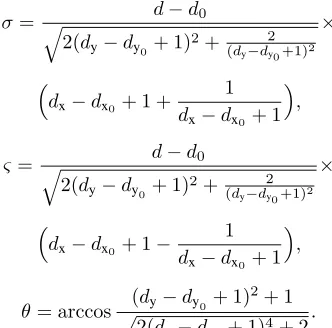
For the suggested model we can easily find the relation between PSF parameters and control variables
σ= q d−d0
2(dy−dy0+ 1)
2+ 2
(dy−dy0+1) 2
×
dx−dx0+ 1 +
1 dx−dx0+ 1
,
ς = q d−d0
2(dy−dy0+ 1)2+(d 2
y−dy0+1) 2
×
dx−dx0+ 1−
1 dx−dx0+ 1
,
θ= arccos (dy−dy0+ 1)
2+ 1
p
2(dy−dy0+ 1)
[image:2.595.342.508.614.778.2](a) (b) (c) (d)
Fig. 2. 2(a): typical configuration of electrostatic stigmators [14]; 2(b): asymmetric PSF in Fourier space, schematic representation; 2(c): The image formation model; 2(d): Sharpness functionSreaches its optimum at the in-focus image. The goal of the autofocus procedure is to find the value of defocus d0.
D. Linear image formation model
Images for which our sharpness function will be computed are the output images f ∈ L2(R2) of the so-called image formation model represented by Figure 2(c). The object’s geometry (or the object function) is denoted byψ. The filter ̺σ describes the PSF of an optical device.
The output of the ̺σ filter is denoted by f0 and is
often processed by a PC. We assume that in such
post-processing a Gaussian filter gα(x) := 2πα12e−
|x|2
2α2 is applied to the image f0. Filtering with a Gaussian kernel is often
used for denoising purposes, which is an easy alternative to more advanced techniques [18], [19], [20]. It has been shown that the control variable αis useful not only for denoising the imagef0; it also influences the approximation error when
the sharpness function is replaced by a quadratic polynomial [13]. The value ofαis fixed during the autofocus process.
We apply the linear image formation model, which is often used for different optical devices [2], in particular for electron microscopes [3]. In this paper we consider low-to-medium magnification of the electron microscope (resolution higher or equal to 1 nm), thus the image formation can be approximated with this model [21]. This implies that the occurring filters are linear and space invariant which can easily be described by means ofconvolutionproducts
f0:=ψ∗̺σ, f :=f0∗gα. (9) If no post-processing is applied,α= 0, andf =f0.
E. Object function
We assume that the object function satisfies
Z Z ∞
−∞|
ψ(x)|dx<∞. (10)
In practice this will easily be satisfied because the function ψ has a finite domain, i.e., the image has a finite size. As a consequenceψˆis bounded and continuous.
In classical signal analysis a discrete signalψis modelled as a finite linear combination of delta functions
ψ(x) = K
X
k,l=1
ak,lδ(x−τk), k:= (k, l)T, τ >0. (11)
We consider the image with a finite number of pixels ak,l, i.e. K < ∞. In this case ψˆ is a tri-geometric polynomial which again is bounded and smooth.
Property 1. The power spectrum of the object function (11)
can be expressed as
|ψˆ(u)|2=X
n,m
ρn,meiτn·u, n:= (n, m)T, (12) where
ρn,m:=
X
k,l
ak,lan+k,m+l, (13)
are theautocorrelationco¨effici¨ents of the pixel values.
Proof: The proof is analogue to the 1-D case [13]. As a special example of an object function consider
|ψˆ(u)|2=Ce−|u|2γ2
, C >0, γ≥0. (14)
Such images, for γ > 0, often occur in real-world appli-cations from single particles. For γ = 0 in (14), |ψˆ|2 is
constant, which corresponds to the situation when the object is nearly amorphous [3].
III. GRADIENT-BASED SHARPNESS FUNCTION
The existing autofocus methods used for different types of optical devices are usually based on asharpness function
S : L2(R2) → R, a real-valued estimate of the image’s
quality. For a through-focus series of images the sharpness function is computed for different values ofdgiven a fixed value of α. A general behaviour of a sharpness function is shown in Figure 2(d). The image at the defocus d = d0
is sharp or in-focus and the sharpness function reaches its optimum. The image far away fromd0is calledout-of-focus.
For simultaneous defocus and astigmatism correction stig-mator controls are ajusted as well, and the goal is to estimate
d0 from the values of the sharpness function computed at
different points.
In this section we provide the general properties of the gradient-based sharpness function
S:=
|∇f|
2
L2. (15)
Property 2. If f is given by (9) with the PSF (7) then the
sharpness function (15) can be written as follows
S(σ) = 1 2π
Z Z ∞
−∞
|u|2|ψˆ(u)|2e−|(RθJσu)
β |2
e−|u|2 α2
du.
(16)
Proof: Because of Parseval’s identity we have
S(σ) = 1 2π
Z Z ∞
−∞|
Corollary 1. The sharpness function can be expressed as
S(σ) = 1 2π
Z Z ∞
−∞|
u|2|ψˆ(u)|2e−σ2β|uβ|2
e−|u|2α2
du. (17)
Corollary 2. The sharpness function is smooth, and is
strictly increasing for σ < 0 and strictly decreasing for σ >0.
Corollary 3. The sharpness function has a finite maximum
atσ= 0 forα >0; in particularmaxσS(σ) =S(0). It follows that the basic properties of the gradient-based sharpness function in 2-D are similar to the properties in 1-D [13], if we consider a rotationally symmetric PSF: for the noise free image formation the function has a unique optimum at the in-focus image. Further we consider the Gaussian PSF (β = 1in (7)).
Property 3. The sharpness function S can be expressed by
means of the autocorrelation co¨effici¨ents (13) as follows
S(σ) = 1 2π(σ2+α2)2
X
n,m ρn,m
Z Z ∞
−∞| u|2e
iτn·u √
α2 +σ2e−|u|2du.
(18)
Proof: After we rewrite the sharpness function (17)
S(σ) = 1 2π(σ2+α2)2
Z Z ∞
−∞|
u|2|ψˆ(√ u
α2+σ2)| 2e−|u|2
du.
and substitute the expression for the power spectrum (12), we achieve (18).
Theorem 1. The sharpness function can be expressed as
S(σ) = C1
2π(α2+σ2)2(1 +R1(σ)), (19)
where
|R1(σ)| ≤K1√ τ
α2+σ2, (20)
andC1, K1 depend only on the pixel valuesak,l.
Proof: Splittinge iτn·u √
α2 +σ2 into(e
iτn·u √
α2 +σ2
−1)+1in (18), one obtains
S(σ) = 1 2π(σ2+α2)2
Z Z ∞
−∞|
u|2e−|u|2 duX
n,m ρn,m
| {z }
C1
+
Z Z ∞
−∞|
u|2e−|u|2X n,m
ρn,m(e iτn·u √
α2 +σ2
−1)du. (21)
It trivially follows that
C1=
Z Z ∞
−∞|
u|2e−|u|2duX
n,m
ρn,m=π
X
n,m ρn,m.
To estimateR1 observe that
|eiη−1|= 2|sinη
2| ≤ |η|, η∈R, (22)
≤√
α2+σ2 |u|
n,m
|n|ρn,m+|v|
n,m
|m|ρn,m . (23)
It follows
Z Z ∞
−∞|
u|2e−|u|2X n,m
ρn,m(e iτn·u √
α2 +σ2
−1)du
≤
≤3
√
π 2
τ
√
α2+σ2
X
n,m
(|n|+|m|)ρn,m.
Then the statement of the theorem is straightforward with
K1= 3 2√π
P
n,m(|n|+|m|)ρn,m
P
n,mρn,m .
It follows from (19) that the function S−1/2(σ) can be
approximated with any accuracy by a quadratic polynomial by increasing the value of the control variableα. This also corresponds to the findings made for the 1-D setting before. The only difference is the power of the sharpness function to be taken for a quadratic approximation. Below we examine a more general case of a non-symmetric PSF.
B. Non-symmetric PSF
Property 4. Image rotation does not influence the sharpness
function, i.e.
S[Rθf] =S[f].
Proof: Rotation transformation is just a linear trans-formation of the coordinates, which satisfies the properties detRθ= 1, R−θT =Rθ, thus
S[Rθf] =k ∂
∂xRθfkL2 =kRθ ∂
∂xfkL2=
1 detRθk
∂ ∂xfkL2.
Corollary 4. For the linear image formation model, the
rotation of the PSF does not influence the sharpness function
S[ψ∗Rθ̺σ∗gα] =S[ψ∗̺σ∗gα].
For further simplification of our analysis we make there-fore a general assumptionθ = 0 in (16). In these case the adjustment of stigmatordy is not necessary. Neglecting the
PSF rotation angle does not limit the theoretical observations. However, in real-world applications defocus and astigmatism correction still remain a three-parameter problem. It has not been possible so far to implement PSF rotation directly in the hardware; thus its elliptic form can be adjusted only by a combination of the two stigmator control variables.
Property 5. For the object function (14) and the Gaussian
PSF the sharpness function (15) is given by
S(σ) = C(ς
2+σ2+α2+γ2)
2(ς2+σ2+α2+γ2)2−4ς2σ23/2
−3 −2 −1 0 1 2 3 100
102
104
106
Blur σ
Sharpness function
(a)ς= 0(astigmatism-free)
−3 −2 −1 0 1 2 3 10−2
10−1
100
101
102
103
104
Blur σ
Sharpness function
[image:5.595.320.529.55.160.2](b)ς= 1(with astigmatism)
Fig. 3. Sharpness functionsSshapes.
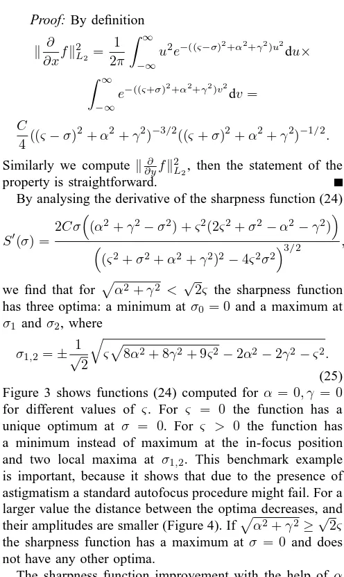
Proof: By definition
k∂x∂ fk2L2=
1 2π
Z ∞
−∞
u2e−((ς−σ)2+α2+γ2)u2du×
Z ∞
−∞
e−((ς+σ)2+α2+γ2)v2dv= C
4((ς−σ)
2+α2+γ2)−3/2((ς+σ)2+α2+γ2)−1/2.
Similarly we compute k∂y∂ fk2L2, then the statement of the property is straightforward.
By analysing the derivative of the sharpness function (24)
S′(σ) =
2Cσ(α2+γ2−σ2) +ς2(2ς2+σ2−α2−γ2)
(ς2+σ2+α2+γ2)2−4ς2σ23/2
,
we find that for pα2+γ2 < √2ς the sharpness function
has three optima: a minimum atσ0= 0 and a maximum at
σ1 andσ2, where
σ1,2=± 1
√
2
q
ςp8α2+ 8γ2+ 9ς2−2α2−2γ2−ς2.
(25) Figure 3 shows functions (24) computed for α= 0, γ = 0 for different values of ς. For ς = 0 the function has a unique optimum at σ = 0. For ς > 0 the function has a minimum instead of maximum at the in-focus position and two local maxima at σ1,2. This benchmark example
is important, because it shows that due to the presence of astigmatism a standard autofocus procedure might fail. For a larger value the distance between the optima decreases, and their amplitudes are smaller (Figure 4). Ifpα2+γ2≥√2ς
the sharpness function has a maximum at σ = 0 and does not have any other optima.
The sharpness function improvement with the help of α adjustments has been shown before experimentally for an electron microscopy through-focus series with local optima due to the astigmatism presence ([13], page 13, Figure 7). The benchmark case, which we studied in this subsection gives a theoretical insight into this effect.
Property 6. For the object function (14) and the Gaussian
PSF the sharpness function in the two-parameter spaceS= S(σ)has a maximum atσ= (0,0)T and does not have any
other optimum.
Proof: It is easy to find that partial derivatives of the function (24)
∂
∂σS(0,0) = ∂
∂ςS(0,0) = 0.
Further it is clear that forς ∈R,∂ς∂ S(σk, ς)6= 0, k= 1,2.
−1 −0.5
0 0.5
1
−1 −0.5 0 0.5 1 2000 4000 6000 8000
σ α=0.1
ς
Sharpness function
−1 −0.5
0 0.5
1
−1 −0.5 0 0.5 1 0.035 0.04 0.045 0.05 0.055 0.06
σ α=2
ς
[image:5.595.58.277.55.146.2]Sharpness function
Fig. 4. Sharpness functionsSshape in a two-parameter space.
Figure 4 shows the sharpness function shape in a two-parameter space computed for α= 0.1 and α= 2. In both cases the sharpness function has a maximum asσ= (0,0)T
and does not have any other optima. This is convenient for simultaneous defocus and astigmatism correction, which could be done by optimizing the sharpness function in two-parameter space [4], [10]: the local optima that the sharpness function obtains in 1-D are not optima anymore in higher dimensions. This funding coincide with the results of the sharpness function behaviour obtained via simulations of the variance-based sharpness function [4]. Still, tuning the artifi-cial blurαmake the shaper of the sharpness function closer to convex, which might increase the speed of optimization.
Corollary below directly follows from Property 2.
Corollary 5. For the Gaussian object function and the
symmetric Gaussian PSF (ς = 0) the sharpness function (15) is given by
S(σ) = C
2(σ2+α2+γ2)2. (26)
In this case the sharpness function to the power−1/2is a quadratic polynomial
S−1/2(d−d0) = 2
r
π
C((d−d0)
2+α2+γ2).
is a quadratic polynomial, which is coincides with the observations of Theorem 1, which are made for a more general case.
IV. AN AUTOMATIC AUTOFOCUS ALGORITHM FOR A REAL-WORLD APPLICATION
A detailed description of the gradient-based fast autofocus method can be found in [13]. Here we just provide a short overview of the autofocus algorithm:
1) Let d2 be the current defocus control value. Choose ∆d, thend1:=d2−∆d, d3:=d3−∆d.
2) Obtain three images at d1, d2, d3 and compute
S1, S2, S3. We set N= 3.
3) We fit N given points with a quadratic polynomial
P(d) :=c0+c1d+c2d2.
ForN >3we obtain the overdetermined system
1 d1 d21
. . . . 1 dN d2N
| {z }
D
c0
c1
c2
| {z }
c
=
S1
. . . SN
| {z }
s
[image:5.595.45.293.179.594.2](a) (b) (c) (d)
−10 −5 0 5
Defocus [µ m]
Sharpness function
[image:6.595.55.535.52.163.2](e)
Fig. 5. Image improvement by a test application implemented in a prototype FEI Tecnai F20 STEM. The plot on the right shows the fitting of the three data points with a quadratic polynomial and thus obtaining of the in-focus image.
This can e.g. be solved by least squares, giving
DTDc=DTs,
computec; estimate the sharpness function optimum
dN+1=−c1 2c2
.
as the optimum of the polynomial
4) If for the given tolerance |dN−dN+1| < dtol, stop. Else, compute SN+1 = S(dN+1) and go to the
previous step.
More iterations (N > 3) are required only if a very accurate focusing is needed. In step three different numerical methods could be used. The choice of the method is not quite significant for small N. For a proper choice of α it can be possible to extend the algorithm to simultaneous autofocus and astigmatism correction by fitting the sharpness function with a quadratic polynomial in a higher dimension.
The autofocus method is implemented in a prototype FEI Tecnai F20 STEM. One example of an application run is shown in Figure 5. The initial position of the machine defocus is d1 = −3 µm. The defocus step ∆d = 5 µm
is chosen. The two intermediate images with d2 =−8 µm
andd3= 2µmare obtained. For each of the imagesS−1/2is
computed. The position of the in-focus image is calculated from the given three images and corresponds to d4 = 0.3
µm, which is within the tolerable defocus error for the given machine settings. The improvements of the image quality are visible in Figure 5. Different examples of our algorithm work for a particle analysis application can be found in [13].
V. DISCUSSION AND CONCLUSIONS
In this paper we have given a better insight into the analytical properties of the gradient-based sharpness function in the 2-D setting. It has been shown that the role of the artificial blur control variable α in the higher dimension becomes more important due to the possible presence of astigmatism. If we only do the autofocus the proper choice of α helps to avoid the multiple optima of the sharpness function. If we perform automated simultaneous defocus and astigmatism correction, by controlling α we can improve the shapes of the sharpness function and increase the speed of optimization. Our results are implemented for real-world applications and deliver a satisfactory performance.
ACKNOWLEDGMENT
We acknowledge R. Doornbos (ESI), S. Sluyterman (FEI), W. Van den Broek (EMAT) for the assistance with experi-ments.
REFERENCES
[1] A. Tejada, S. van der Hoeven, A. den Dekker, and P. Van den Hof, “Towards automatic control of scanning transmission electron microscopes,” in Proc. 18th IEEE International Conference on Control
Applications, 2009, pp. 788–793.
[2] S. K. Nayar and Y. Nakagawa, “Shape from focus,” IEEE Trans.
Pattern Anal. Mach. Intell., vol. 16, no. 8, pp. 824–831, 1994.
[3] S. Erasmus and K. Smith, “An automatic focusing and astigmatism correction system for the SEM and CTEM,” J. Microsc., vol. 127, no. 2, pp. 185–199, 1982.
[4] M. Rudnaya, W. Van den Broek, R. Doornbos, R. Mattheij, and J. Maubach, “Autofocus and twofold astigmatism correction in HAADF-STEM,” Ultramicroscopy, vol. accepted, doi:10.1016/j.ultramic.2011.01.034, 2011.
[5] D. Vollath, “Automatic focusing by correlative methods,” J. Microsc., vol. 147, pp. 279–288, Sep 1987.
[6] E. Krotkov, “Focusing,” Int. J. Comput. Vis., vol. 1, pp. 223–237, 1987. [7] S. Jutamulia, T. Asakura, R. Bahuguna, and C. De Guzman, “Aut-ofocusing based on power-spectra analysis,” Applied optics, vol. 33, no. 26, pp. 6210–6212, 1994.
[8] T. Yeo, S. Ong, Jayasooriah, and R. Sinniah, “Autofocusing for tissue microscopy,” Image Vis. Comput., vol. 11, no. 10, pp. 629–639, 1993. [9] M. Rudnaya, R. Mattheij, and J. Maubach, “Evaluating sharpness functions for automated scanning electron microscopy,” J. Microsc., vol. 240, pp. 38–49, 2010.
[10] M. Rudnaya, S. Kho, R. Mattheij, and J. Maubach, “Derivative-free optimization for autofocus and astigmatism correction in electron microscopy,” in Proc. 2nd International Conference on Engineering
Optimization, Lisbon, Portugal, 2010.
[11] P. Van Bree, C. Van Lierop, and P. Van den Bosch, “On hysteresis in magnetic lenses of electron microscopes,” in Proc. ISIE, Bari, Italy, 2010.
[12] M. Rudnaya, R. Mattheij, and J. Maubach, “Iterative autofocus algo-rithms for scanning electron microscopy,” Microsc. Microanal., vol. 15(Suppl 2), pp. 1108–1109, 2009.
[13] M. Rudnaya, H. ter Morsch, J. Maubach, and R. Mattheij, “A derivative-based fast autofocus method,” Eindhoven University of Technology, CASA-report 11-13, 2011, http://www.win.tue.nl/analysis/reports/rana11-13.pdf.
[14] K. Ong, J. Phang, and J. Thong, “A robust focusing and astigmatism correction method for the scanning electron microscope,” Scanning, vol. 19, pp. 553–563, 1997.
[15] W. Riecke, Topics in Current Physics: Magnetic Electron Lenses. Spring-Verlag, 1982, ch. Practical lens design, pp. 164–351. [16] A. Carasso, D. Bright, and A. Vladar, “APEX method and real-time
blind deconvolution of scanning electron microscopy imagery,” Opt.
Eng, vol. 41, no. 10, pp. 2499–2514, 2002.
[17] C. Johnson, “A method for characterizing electro-optical device modu-lation transfer function,” Photograph. Sci. Eng., vol. 14, no. 413–415, 1970.
[18] S. Morigi, L. Reichel, F. Sgallari, and A. Shyshkov, “Cascadic mul-tiresolution methods for image deblurring,” SIAM J. Imaging Sci., vol. 1, no. 1, pp. 51–74, 2007.
[19] K. Kumar, M. Pisarenco, M. Rudnaya, V. Savcenco, and S. Srivastava, “Shape reconstruction techniques for optical sectioning of arbitrary objects,” Mathematics–in–Industry case studies, vol. accepted, 2011. [20] T. Le, R. Chartrand, and T. Asaki, “A variational approach to
recon-structing images corrupted by poisson noise,” J. Math. Imaging Vis., vol. 27, no. 3, pp. 257–263, 2007.
![Fig. 2.2(a): typical configuration of electrostatic stigmators [14]; 2(b): asymmetric PSF in Fourier space, schematic representation; 2(c): The imageformation model; 2(d): Sharpness function S reaches its optimum at the in-focus image](https://thumb-us.123doks.com/thumbv2/123dok_us/1288370.657805/3.595.59.537.54.160/conguration-electrostatic-stigmators-asymmetric-schematic-representation-imageformation-sharpness.webp)