Sample Selection for Statistical Parsing

Rebecca Hwa

Corpus-based statistical parsing relies on using large quantities of annotated text as training examples. Building this kind of resource is expensive and labor-intensive. This work proposes to use sample selection to find helpful training examples and reduce human effort spent on annotating less informative ones. We consider several criteria for predicting whether unlabeled data might be a helpful training example. Experiments are performed across two syntactic learning tasks and within the single task of parsing across two learning models to compare the effect of different predictive criteria. We find that sample selection can significantly reduce the size of annotated training corpora and that uncertainty is a robust predictive criterion that can be easily applied to different learning models.

1. Introduction

Many learning tasks for natural language processing require supervised training; that is, the system successfully learns a concept only if it has been given annotated train-ing data. For example, while it is difficult to induce a grammar with raw text alone, the task is tractable when the syntactic analysis for each sentence is provided as a part of the training data (Pereira and Schabes 1992). Current state-of-the-art statisti-cal parsers (Collins 1999; Charniak 2000) are all trained on large annotated corpora such as the Penn Treebank (Marcus, Santorini, and Marcinkiewicz 1993). However, supervised training data are difficult to obtain; existing corpora might not contain the relevant type of annotation, and the data might not be in the domain of interest. For example, one might need lexical-semantic analyses in addition to the syntactic anal-yses in the treebank, or one might be interested in processing languages, domains, or genres for which there are no annotated corpora. Because supervised training de-mands significant human involvement (e.g., annotating the syntactic structure of each sentence by hand), creating a new corpus is a labor-intensive and time-consuming en-deavor. The goal of this work is to minimize a system’s reliance on annotated training data.

One promising approach to mitigating the annotation bottleneck problem is to usesample selection, a variant of active learning. Sample selection is an interactive learning method in which the machine takes the initiative in selecting unlabeled data for the human to annotate. Under this framework, the system has access to a large pool of unlabeled data, and it has to predict how much it can learn from each candidate in the pool if that candidate is labeled. More quantitatively, we associate each candidate in the pool with a training utility value(TUV). If the system can accurately identify the subset of examples with the highest TUV, it will have located the most beneficial

∗Computer Science Department, Pittsburgh, PA 15260. E-mail: [email protected].

training examples, thus freeing the annotators from having to label less informative examples.

In this article, we apply sample selection to two syntactic learning tasks: training a prepositional-phrase attachment (PP-attachment) model and training a statistical parsing model. We are interested in addressing two main questions. First, what are good predictors of a candidate’s training utility? We propose several predictive criteria and define evaluation functions based on them to rank the candidates’ utility. We have performed experiments comparing the effect of these evaluation functions on the size of the training corpus. We find that, with a judiciously chosen evaluation function, sample selection can significantly reduce the size of the training corpus. The second main question is: Are the predictors consistently effective for different types of learners? We compare the predictive criteria both across tasks (between PP-attachment and parsing) and within a single task (applying the criteria to two parsing models: an expectation-maximization-trained parser and a count-based parser). We find that the learner’s uncertainty is a robust predictive criterion that can be easily applied to different learning models.

2. Learning with Sample Selection

Unlike traditional learning systems that receive training examples indiscriminately, a sample selection learning system actively influences its own progress by choosing new examples to incorporate into its training set. There are two types of selection algo-rithms: committee-based andsingle learner. A committee-based selection algorithm works with multiple learners, each maintaining a different hypothesis (perhaps per-taining to different aspects of the problem). The candidate examples that lead to the most disagreements among the different learners are considered to have the highest TUV (Cohn, Atlas, and Ladner 1994; Freund et al. 1997). For computationally intensive problems, such as parsing, keeping multiple learners may be impractical.

In this work, we focus on sample selection using a single learner that keeps one working hypothesis. Without access to multiple hypotheses, the selection algorithm can nonetheless estimate the TUV of a candidate. We identify the following three classes of predictive criteria:

1. Problem-space:Knowledge about the problem space may provide

information about the type of candidates that are particularly plentiful or difficult to learn. This criterion focuses on the general attributes of the learning problem, such as the distribution of the input data and properties of the learning algorithm, but it ignores the current state of the hypothesis.

2. Performance of the hypothesis:Testing the candidates on the current working hypothesis shows the type of input data on which the hypothesis may perform weakly. That is, if the current hypothesis is unable to label a candidate or is uncertain about it, then the candidate might be a good training example (Lewis and Catlett 1994). The

underlying assumption is that an uncertain output is likely to be wrong.

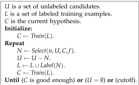
Uis a set of unlabeled candidates. L is a set of labeled training examples. Cis the current hypothesis.

Initialize:

C←Train(L).

Repeat

N←Select(n,U,C,f). U←U−N.

L←L∪Label(N). C←Train(L).

Until(Cis good enough)or(U=∅)or(cutoff).

Figure 1

Pseudo code for the sample selection learning algorithm.

Figure 1 outlines the single-learner sample selection training loop in pseudocode. Initially, the training set, L, consists of a small number of labeled examples, based on which the learner proposes its first hypothesis of the target concept,C. Also available to the learner is a large pool of unlabeled training candidates, U. In each training iteration, the selection algorithm,Select(n,U,C,f), ranks the candidates ofUaccording to their expected TUVs and returns the n candidates with the highest values. The algorithm predicts the TUV of each candidate, u ∈ U, with an evaluation function, f(u,C). This function may rely on the hypothesis conceptCto estimate the utility of a candidate u. Then chosen candidates are then labeled by human experts and added to the existing training set. Running the learning algorithm,Train(L), on the updated training set, the system proposes a new hypothesis regarding the target concept that is the most compatible with the examples seen thus far. The loop continues until one of three stopping conditions is met: The hypothesis is considered to perform well enough, all candidates are labeled, or an absolute cutoff point is reached (e.g., no more resources).

3. Sample Selection for Prepositional-Phrase Attachment

One common source of structural ambiguities arises from syntactic constructs in which a prepositional phrase might be equally likely to modify the verb or the noun pre-ceding it. Researchers have proposed many computational models for resolving PP-attachment ambiguities. Some well-known approaches include rule-based models (Brill and Resnik 1994), backed-off models (Collins and Brooks 1995), and a maximum-entropy model (Ratnaparkhi 1998). Following the tradition of using learning PP-attachment as a way to gain insight into the parsing problem, we first apply sample selection to reduce the amount of annotation used in training a PP-attachment model. We use the Collins-Brooks model as the basic learning algorithm and experiment with several evaluation functions based on the types of predictive criteria described earlier. Our experiments show that the best evaluation function can reduce the number of labeled examples by nearly half without loss of accuracy.

3.1 A Summary of the Collins-Brooks Model

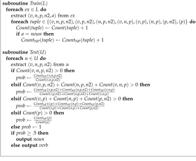
subroutineTrain(L) foreachex∈L do

extract(v,n,p,n2,a)fromex

foreachtuple∈ {(v,n,p,n2),(v,p,n2),(n,p,n2),(v,n,p),(v,p),(n,p),(p,n2),(p)}do

Count(tuple)←Count(tuple) +1

ifa=nounthen

CountNP(tuple)←CountNP(tuple) +1

subroutineTest(U) foreachu∈Udo

extract(v,n,p,n2)fromu

ifCount(v,n,p,n2)>0 then

prob← CountNP(v,n,p,n2)

Count(v,n,p,n2)

elsifCount(v,p,n2) +Count(n,p,n2) +Count(v,n,p)>0then

prob← CountNP(v,p,n2)+CountNP(n,p,n2)+CountNP(v,n,p)

Count(v,p,n2)+Count(n,p,n2)+Count(v,n,p)

elsifCount(v,p) +Count(n,p) +Count(p,n2)>0then

prob← CountNP(v,p)+CountNP(n,p)+CountNP(p,n2)

Count(v,p)+Count(n,p)+Count(p,n2) elsifCount(p)>0 then

prob← CountNP(p)

Count(p) elseprob←1

ifprob≥.5then outputnoun

else outputverb

Figure 2

The Collins-Brooks PP-attachment classification algorithm.

preposition, and the prepositional noun phrase, respectively, andaspecifies the attach-ment classification. For example, (wrote a book in three days, attach-verb) would be anno-tated as(wrote,book,in,days,verb). The head words can be automatically extracted using a heuristic table lookup in the manner described by Magerman (1994). For this learning problem, the supervision is the one-bit information of whetherpshould attach tovor ton. In order to learn the attachment preferences of prepositional phrases, the system builds attachment statistics for each thecharacteristic tupleof all training examples. A characteristic tuple is some subset of the four head words in the example, with the con-dition that one of the elements must be the preposition. Each training example forms eight characteristic tuples:(v,n,p,n2),(v,n,p),(v,p,n2),(n,p,n2),(v,p),(n,p),(p,n2),(p). The attachment statistics are a collection of the occurrence frequencies for all the char-acteristic tuples in the training set and the occurrence frequencies for the charchar-acteristic tuples of those examples determined to attach to nouns. For some characteristic tuple t,Count(t)denotes the former andCountNP(t)denotes the latter. In terms of the sample

selection algorithm, the collection of counts represents the learner’s current hypothesis (Cin Figure 1). Figure 2 provides the pseudocode for theTrainroutine.

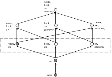
Figure 3

In this example, the classification of the test case preposition is backed off to the

two-word-tuple level. In the diagram, each circle represents a characteristic tuple. A filled circle denotes that the tuple has occurred in the training set. The dashed rectangular box indicates the back-off level on which the classification is made.

never occurred in the training example, the classifier would then back off to look at the test case’s three three-word characteristic tuples. It would continue to back off further, if necessary. In the case that the model has no information on any of the characteristic tuples of the test case, it would, by default, classify the test case as an instance of noun attachment. Figure 3 shows using the back-off scheme on a test case. We describe in theTest pseudocode routine in Figure 2 the model’s classification procedure for each back-off level.

3.2 Evaluation Functions

Based on the three classes of predictive criteria discussed in Section 2, we propose several evaluation functions for the Collins-Brooks model.

3.2.1 The Problem Space. One source of knowledge to exploit is our understanding of the PP-attachment model and properties of English prepositional phrases. For instance, we know that the most problematic test cases for the PP-attachment model are those for which it has no statistics at all. Therefore, those data that the system has not yet encountered might be good candidates. The first evaluation function we define,

fnovel(u,C), equates the TUV of a candidate u with its degree of novelty, the number

of its characteristic tuples that currently have zero counts:1

fnovel(u,C) =

t∈Tuples(u)

1 : Count(t) =0 0 : otherwise

This evaluation function has some blatant defects. It may distort the data distribution so much that the system will not be able to build up a reliable collection of statistics. The function does not take into account the intuition that those data that rarely occur, no matter how novel, probably have overall low training utility. Moreover, the scoring scheme does not make any distinction between the characteristic tuples of a candidate.

book, on, shelf book, on, put, book, on, shelf put, on, shelf put, on, on, book, shelf on, put, noun on, on, shelf put, on, shelf on, put, idea on, noun put, on, shelf put, on, shelf on, on, idea idea idea book, shelf on, on, wrote on, noun book, on, shelf book, on, on, shelf shelf book, on, on, wrote wrote wrote idea on, noun on, on, on, on, on, topic had idea on, topic topic topic idea had on, had idea had topic

u1, u2 u3 u4 u5

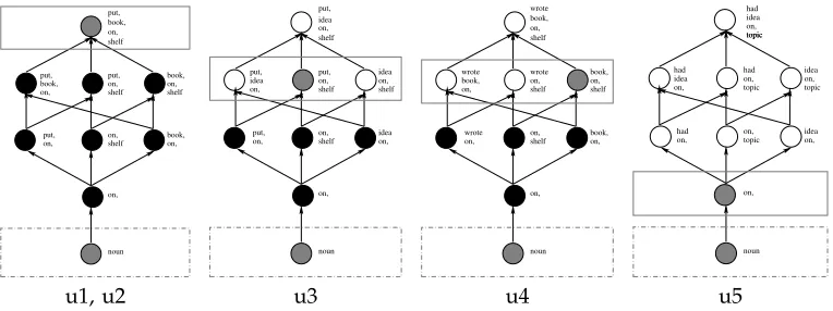
Figure 4

If candidateu1 is selected, a total of 22 tuples can be ignored. The dashed rectangles show the

classification level before training, and the solid rectangles show the classification level after

the statistics ofu1 have been taken. The obviated tuples are represented by the filled black

circles.

We know, however, that the PP-attachment classifier is a back-off model that makes its decision based first on statistics of the characteristic tuple with the most words. A more sophisticated sampling of the data domain should consider not only the novelty of the data, but also the frequency of its occurrence, as well as the quality of its charac-teristic tuples. We define a back-off-model-based evaluation function,fbackoff(u,C), that

scores a candidate u by counting the number of characteristic tuples that would be obviated in all candidates ifuwere included in the training set. For example, suppose we have a small pool of five candidates, and we are about to pick the first training example:

u1 = (put, book, on, shelf)

u2 = (put, book, on, shelf)

u3 = (put, idea, on, shelf)

u4 = (wrote, book, on, shelf)

u5 = (had, idea, on, topic)

According to fbackoff, either u1 or u2 would be the best choice. By selecting either as

the first training example, we could ignore all but the four-word characteristic tuple for both u1 and u2 (a saving of seven tuples each); since u3 and u4 each have three

words in common with the first two candidates, they would no longer depend on their lower four tuples; and although we would also improve the statistics for one of u5’s tuples (on), nothing could be pruned from u5’s characteristic tuples. Thus,

fbackoff(u1,C) =fbackoff(u2,C) =7+7+4+4=22 (see Figure 4).

Underfbackoff, ifu1 were chosen as the first example,u2 would lose all its utility,

because we could not prune any extra characteristic tuples by using u2. That is, in

the next round of selection,fbackoff(u2,C) =0. Candidateu5 would be the best second

example because it would now have the most tuples to prune (7 tuples).

The evaluation functionfbackoff improves uponfnovelin two ways. First, novel

after selecting u1 as the first training example, we would no longer care about the

two-word tuples ofu4 such as (wrote, on), even though we have no statistics for them.

A potential problem withfbackoffis that after all the obvious candidates have been

selected, the function is not very good at differentiating between the remaining can-didates that have about the same level of novelty and occur infrequently.

3.2.2 The Performance of the Hypothesis. The evaluation functions discussed in the previous section score candidates based on prior knowledge alone, independent of the current state of the learner’s hypothesis and the annotation of the selected training examples. To attune the selection of training examples to the learner’s progress, an evaluation function might factor in its current hypothesis in predicting a candidate’s TUV.

One way to incorporate the current hypothesis into the evaluation function is to score each candidate using the current model, assuming its hypothesis is right. An error-driven evaluation function, ferr, equates the TUV of a candidate with the

hypothesis’ estimate of its likelihood to misclassify that candidate (i.e., one minus the probability of the most-likely class). If the hypothesis predicts that the likelihood of a prepositional phrase to attach to the noun is 80%, and if the hypothesis is accurate, then there is a 20% chance that it has misclassified.

A related evaluation function is one that measures the hypothesis’s uncertainty

across all classes, rather than focusing on only the most likely class. Intuitively, if the hypothesis classifies a candidate as equally likely to attach to the verb as to the noun, it is the most uncertain of its answer. If the hypothesis assigns a candidate to a class with a probability of one, then it is the most certain of its answer. For the binary-class case, the uncertainty-based evaluation function, func, can be expressed in the same way as

the error-driven function, as a function that is symmetric about 0.5 and monotonically decreases if the hypothesis prefers one class over another:2

func(u,C) = ferr(u,C)

=

1−P(noun|u,C) : P(noun|u,C)≥0.5 P(noun |u,C) : otherwise

= 0.5−abs(0.5−P(noun |u,C)) (1)

In the general case of choosing between multiple classes,ferrandfuncare different from

one another. We shall return to this point in Section 4.1.2 when we consider training parsers.

The potential drawback of the performance-based evaluation functions is that they assume that the hypothesis is correct. Selecting training examples based on a poor hy-pothesis is prone to pitfalls. On the one hand, the hyhy-pothesis may be overly confident about the certainty of its decisions. For example, the hypothesis may assign nounto a candidate with a probability of one based on parameter estimates computed from a single previous observation in which a similar example was labeled asnoun. Despite the unreliable statistics, this candidate would not be selected, since the hypothesis considers this a known case. Conversely, the hypothesis may also direct the selec-tion algorithm to chase after undecidable cases. For example, consider preposiselec-tional phrases (PPs) withinas the head. These PPs occur frequently, and about half of them should attach to the object noun. Even though training on more labeled in examples

does not improve the model’s performance on future in PPs, the selection algorithm will keep on requesting moreintraining examples because the hypothesis remains un-certain about this preposition.3 _{With an unlucky starting hypothesis, these evaluation} functions may select uninformative candidates initially.

3.2.3 The Parameters of the Hypothesis. The potential problems with performance-based evaluation function stems from their trust in the model’s diagnosis of its own progress. Another way to incorporate the current hypothesis is to determine how good it is and what type of examples will improve it the most. In this section we propose an evaluation function that scores candidates based on their utilities in increasing the confidence about the parameters of the hypothesis (i.e., the collection of statistics over the characteristic tuples of the training examples).

Training the parameters of the PP-attachment model is similar to empirically de-termining the bias of a coin. We measure the coin’s bias by repeatedly tossing it and keeping track of the percentage of times it lands on heads. The more trials we perform, the more confident we become about our estimation of the bias. Similarly, in estimating p, the likelihood of a PP’s attaching to its object noun, we are more confident about the classification decision based on statistics with higher counts than based on statistics with lower counts. A quantitative measurement of our confidence in a statistic is the

confidence interval. This is a region around the measured statistic, bounding the area within which the true statistic may lie. More specifically, the confidence interval forp, a binomial parameter, is defined as

conf int(¯p,n) = 1

1+t_n2

¯

p+ t

2

2n ±t

¯

p(1−¯p)

n +

t2

4n2

where ¯p is the expected value of p based onn trials, andt is athreshold value that depends on the number of trials and the level of confidence we desire. For instance, if we want to be 90% confident that the true statisticp lies within the interval, and ¯_p

is based on n=30 trials, then we settto be 1.697.4 _{Applying the confidence interval} concept to evaluating candidates for the back-off PP-attachment model, we define a function fconf that scores a candidate by taking the average of the lengths of the

confidence interval of each back-off level. That is,

fconf(u,C) = 4

l=1

|conf int(¯pl(u,C),nl(u,C))| 4

where¯pl(u,C)is the probability that modelCwill attachutonounat back-off levell, andnl(u,C)is the number of training examples upon which this classification is based. The confidence-based evaluation function has several potential problems. One of its flaws is similar to that of fnovel. In the early stage, fconf picks the same examples

3 This phenomenon is particularly acute in the early stages of refining the hypothesis because most decisions are based on statistics of the head preposition alone; in the later stages, the hypothesis can usually rely on higher-ordered characteristic tuples that tend to be better classifiers.

asfnovel, because we have no confidence in the statistics of novel examples. Therefore,

fconf is also prone to chase after examples that rarely occur to build up the confidence

of some unimportant parameters. A second problem is thatfconf ignores the output of

the model. Thus, if candidate A has a confidence interval around[0.6, 1]and candidate B has a confidence interval around [0.4, 0.7], then fconf will prefer candidate A, even

though training on A will not change the hypothesis’s performance, since the entire confidence interval is already in the nounzone.

3.2.4 Hybrid Function. The three categories of predictive criteria discussed above are complementary, each focusing on a different aspect of the learner’s weakness. There-fore, it may be beneficial to combine these criteria into one evaluation function. For instance, the deficiency of the confidence-based evaluation function described in the previous section can be avoided if the confidence interval covering the region around the uncertainty boundary (candidate B in the example just discussed) is weighed more heavily than one around the end points (candidate A).

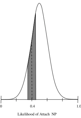
In this section, we introduce a new function that tries to factor in both the uncer-tainty of the model performance and the confidence of the model parameters. First, we define a function, called area(¯p,n), that computes the area under a Gaussian function N(x,µ,σ)with a mean of 0.5 and a standard deviation of 0.1 that is bounded by the confidence interval as computed by conf int(¯p,n) (see Figure 5).5 _{That is, suppose ¯p} has a confidence interval of[a,b]; then

area(¯p,n) =

_b

a

N(x, 0.5, 0.1)dx

Computing area for each back-off level, we define an evaluation function, farea(u,C),

as their average. This function can be viewed as a product offconf andfunc.6

3.3 Experimental Comparison

To determine the relative merits of the proposed evaluation functions, we compare the learning curve of training with sample selection according to each function against a baseline of random selection in an empirical study. The corpus for this comparison is a collection of phrases extracted from the Wall Street Journal (WSJ) Treebank. We use Section 00 as the development set and Sections 2-23 as the training and test sets. We perform 10-fold cross-validation to ensure the statistical significance of the results. For each fold, the training candidate pool contains about 21,000 phrases, and the test set contained about 2,000 phrases.

As shown in Figure 1, the learner generates an initial hypothesis based on a small set of training examples, L. These examples are randomly selected from the pool of unlabeled candidates and annotated by a human. Random sampling ensures that the initial trained set reflects the distribution of the candidate pool and thus that the initial hypothesis is unbiased. Starting with an unbiased hypothesis is important for those evaluation functions whose scoring metrics are affected by the accuracy of the hypothesis. In these experiments,Linitially contains 500 randomly selected examples. In each selection iteration, all the candidates are scored by the evaluation function, andnexamples with the highest TUVs are picked out fromUto be labeled and added

5 The standard deviation value for the Gaussian is chosen so that more than 98% of the mass of the distribution is between 0.25 and 0.75.

0.4

Likelihood of Attach NP

1.0 0

Figure 5

An example: Suppose that the candidate has a likelihood of 0.4 for noun attachment and a

confidence interval of width 0.1. Thenareacomputes the area bounded by the confidence

interval and the Gaussian curve.

toL. Ideally, we would like to haven=1 for each iteration. In practice, however, it is often more convenient for the human annotator to label data in larger batches rather than one at a time. In these experiments, we use a batch size ofn=500 examples.

We make note of one caveat to this kind of n-best batch selection. Under a hypothesis-dependent evaluation function, identical examples will receive identical scores. Because identical (or very similar) examples tend to address the same defi-ciency in the hypothesis, addingnvery similar examples to the training set is unlikely to lead to big improvements in the hypothesis. To diversify the examples in each batch, we simulate single-example selection (whenever possible) by reestimating the scores of the candidates after each selection. Suppose we have just chosen to add candidate x to the batch. Then, before selecting the next candidate, we estimate the potential decrease in scores of candidates similar toxonce it belongs to the annotated training set. The estimation is based entirely on the knowledge that x is chosen, but not on the classification of x. Thus, only certain types of evaluation functions are amenable to the reestimation process. For example, if scores have been assigned by fconf, then

we know that the confidence intervals of the candidates similar to x must decrease slightly after learningx. On the other hand, if scores have been assigned byfunc, then

we cannot perceive any changes in the scores of similar candidates without knowing the true classification of x.

3.3.1 Results and Discussion. This section presents the empirical measurements of the model’s performances using training examples selected by different evaluation functions. We compare each proposed function with the baseline of random selection (frand). The results are graphically depicted from two perspectives. One (e.g., Figure

74 76 78 80 82 84 86

0 5000 10000 15000 20000

Classification accuracy on the test set (%)

Number of examples in the training set baseline

novelty backoff

74 76 78 80 82 84 86

0 5000 10000 15000 20000

Classification accuracy on the test set (%)

Number of examples in the training set

baseline uncertainty confidence

(a) (b)

74 76 78 80 82 84 86

0 5000 10000 15000 20000

Classification accuracy on the test set (%)

Number of examples in the training set baseline

area

0 5,000 10,000 15,000 20,000 25,000

base line

nove lty

backof f

unce rtainty

conf idence ar

ea

Evaluation Functions

Number of Labeled Training Examples

(c) (d)

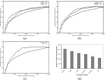
Figure 6

A comparison of the performance of different evaluation functions: (a) compares the learning

curves of the functions that use knowledge about the problem space (fnovelandfbackoff) with

that of the baseline; (b) compares the learning curves of performance-based function (funcand

fconf) with the baseline; (c) compares the learning curve offarea, which combines uncertainty

and confidence, withfunc,fconf, and the baseline; (d) compares all the functions for the number

of training examples selected at the final performance level (83.8%).

functions at the highest performance level. The graph shows that in order to train a model that attaches PPs with an accuracy rate of 83.8%, sample selection with fnovel

requires 2,500 fewer examples than the baseline.

Compared tofnovel,fbackoffselects more helpful training examples in the early stage.

As shown in Figure 6(a), the improvement rate of the model under fbackoff is always

at least as fast that for asfnovel. However, the differences between these two functions

become smaller for higher performance levels. This outcome validates our predictions. Scoring candidates by a combination of their novelty, occurrence frequencies, and the qualities of their characteristic tuples,fbackoffselects helpful early (the first 4,000 or so)

training examples. Then, just as in fnovel, the learning rate remains stagnant for the

next 2,000 poorly selected examples. Finally, when the remaining candidates all have similar novelty values and contain mostly characteristic tuples that occur infrequently, the selection becomes random.

Figure 6(b) compares the two evaluation functions that score candidates based on the current state of the hypothesis. Although both functions suffer a slow start, they are more effective thanfbackoffat reducing the training set when learning high-quality

models. Initially, because all the unknown statistics are initialized to 0.5, selection based onfuncis essentially random sampling. Only after the hypothesis becomes sufficiently

informed selections. Following a similar but more exaggerated pattern, the confidence-based function, fconf, also improves slowly at the beginning before finally overtaking

the baseline. As we noted earlier, because the hypothesis is not confident about novel candidates,fconf andfnoveltend to select the same early examples. Therefore, the early

learning rate offconfis as poor as that offnovel. In the later stage, whilefnovelcontinues

to flounder,fconf can select better candidates based on a more reliable hypothesis.

Finally, the best-performing evaluation function is the hybrid approach. Figure 6(c) shows that the learning curve of farea combines the earlier success offunc and the

later success of fconf to always outperform the other functions. As shown in Figure

6(d), it requires the least number of examples to achieve the highest performance level of 83.8%. Compared to the baseline,farea requires 47% fewer examples to achieve this

performance level. From these comparison studies, we conclude that involving the hypothesis in the selection process is a key factor in reducing the size of the training set.

4. Sample Selecting for Statistical Parsing

In applying sample selection to training a PP-attachment model, we have observed that all effective evaluation functions make use of the model’s current hypothesis in estimating the training utility of the candidates. Although knowledge about the prob-lem space seems to help sharpening the learning curve initially, overall, it is not a good predictor. In this section, we investigate whether these observations hold true for train-ing statistical parstrain-ing models as well. Moreover, in order to determine whether the performances of the predictive criteria are consistent across different learning models within the same domain, we have performed the study on two parsing models: one based on a context-free variant of tree-adjoining grammars (Joshi, Levy, and Taka-hashi 1975), the Probabilistic Lexicalized Tree Insertion Grammar (PLTIG) formalism (Schabes and Waters 1993; Hwa 1998), and Collins’s Model 2 parser (1997). Although both models are lexicalized, statistical parsers, their learning algorithms are different. The Collins Parser is a fully supervised, history-based learner that models the pa-rameters of the parser by taking statistics directly from the training data. In contrast, PLTIG’s expectation-maximization-based induction algorithm is partially supervised; the model’s parameters are estimated indirectly from the training data.

As a superset of the PP-attachment task, parsing is a more challenging learning problem. Whereas a trained PP-attachment model is a binary classifier, a parser must identify the correct syntactic analysis out of all possible parses for a sentence. This classification task is more difficult than PP-attachment, since the number of possible parses for a sentence grows exponentially with respect to its length. Consequently, the annotator’s task is more complex. Whereas the person labeling the training data for PP-attachment reveals one unit of information (always choosing betweennounor verb), the annotation needed for parser training is usually greater than one unit,7 _and the type of labels varies from sentence to sentence. Because the annotation complexity differs from sentence to sentence, the evaluation functions must strike a balance be-tween maximizing potential informational gain and minimizing the expected amount

of annotation exerted. We propose a set of evaluation functions similar in spirit to those for the PP-attachment learner, but extended to accommodate the parsing domain.

4.1 Evaluation Functions

4.1.1 Problem Space. Similarly to scoring a PP candidate based on the novelty and frequencies of its characteristic tuples, we define an evaluation function,flex(w,G)that

scores a sentence candidate, w, based on the novelty and frequencies of word pair co-occurrences:

flex(w,G) =

wi,wj∈wnew(wi,wj)×coocc(wi,wj)

length(w)

where w is the unlabeled sentence candidate,Gis the current parsing model (which is ignored by problem-space-based evaluation functions), new(wi,wj) is an indicator function that returns one if we have not yet selected any sentence in whichwi andwj co-occurred, andcoocc(wi,wj)is a function that returns the number of times thatwi co-occurs8 _{withwjin the candidate pool. We expect these evaluation functions to be less} relevant for the parsing domain than for the PP-attachment domain for two reasons. First, because we do not have the actual parses, the extraction of lexical relationships is based on co-occurrence statistics, not syntactic relationships. Second, because the distribution of words that form lexical relationships is wider and more uniform than that of words that form PP characteristic tuples, most word pairs will be novel and appear only once.

Another simple evaluation function based on the problem space is one that esti-mates the TUV of a candidate from its sentence length:

flen(w,G) =length(w)

The intuition behind this function is based on the general observation that longer sentences tend to have complex structures and introduce more opportunities for am-biguous parses. Although these evaluation functions may seem simplistic, they have one major advantage: They are easy to compute and require little processing time. Because inducing parsing models demands significantly more time than inducing PP-attachment models, it becomes more important that the evaluation functions for pars-ing models be as efficient as possible.

4.1.2 The Performance of the Hypothesis. We previously defined two performance-based evaluation functions: ferr, the model’s estimate of the likelihood that is has

made a classification error, andfunc, the model’s estimate of its uncertainty in making the classification. We have shown the two functions to have similar performance for the PP-attachment task. This is not the case for statistical parsing, however, because the number of possible classes (parse trees) differs from sentence to sentence. For example, suppose we wish to compare one candidate for which the current parsing model generated four equally likely parses with another candidate for which the model generated 1 parse with probability of 0.2 and 99 other parses with a probability of 0.01 (such that they sum to 0.98). The error-driven function,ferr, would score the latter

candidate higher because its most likely parse has a lower probability than that of the most likely parse of the former candidate; the uncertainty-based function,func, would

score the former candidate higher because the model does not have a strong preference

for one parse over any other. In this section, we provide a formal definition for both functions.

Suppose that a parsing modelGgenerates a candidate sentencewwith probability P(w|G), and that the setV contains all possible parses thatGgenerated forw. Then, we denote the probability of G’s generating a single parse,v∈ V, asP(v|G)such that v∈V

P(v|G) =P(w|G). The parse chosen forw is the most likely parse inV, denoted asvmax, where

vmax=argmax_v∈VP(v|G)

Note that P(v | G) reflects the probability of one particular parse tree, v, out of all possible parse trees for all possible sentences that G can generate. To compute the likelihood of a parse’s being the correct parse out of the possible parses ofwaccording toG, denoted asP(v|w,G), we need to normalize the tree probability by the sentence probability. So according toG, the likelihood thatvmaxis the correct parse for wis9

P(vmax|w,G) =

P(vmax|G)

P(w|G) = P(vmax|G)

v∈VP(v|G)

. (2)

Therefore, the error-driven evaluation function is defined as

ferr(w,G) =1−P(vmax|w,G)

Unlike the error-driven function, which focuses on the most likely parse, the uncertainty-based function takes the probability distribution of all parses into account. To quantitatively characterize its distribution, we compute the entropy of the distri-bution. That is,

H(V) =−

v∈V

p(v)lg(p(v)) (3)

whereVis a random variable that can take any possible outcome in setV, andp(v) =

Pr(V=v)is the density function. Further details about the properties of entropy can be found in textbooks on information theory (e.g., Cover and Thomas 1991).

Determining the parse tree for a sentence from a set of possible parses can be viewed as assigning a value to a random variable. Thus, a direct application of the entropy definition to the probability distribution of the parses for sentence w in G computes its tree entropy,TE(w,G), the expected number of bits needed to encode the distribution of possible parses for w. However, we may not wish to compare two sentences with different numbers of parses by their entropy directly. If the parse probability distributions for both sentences are uniform, the sentence with more parses will have a higher entropy. Because longer sentences typically have more parses, using entropy directly would result in a bias toward selecting long sentences. To normalize for the number of parses, the uncertainty-based evaluation function,func, is defined as

a measurement of similarity between the actual probability distribution of the parses and a hypothetical uniform distribution for that set of parses. In particular, we divide

the tree entropy by the log of the number of parses:10

func(w,G) =

TE(w,G)

lg(V)

We now derive the expression for TE(w,G). Recall from equation (2) that if G produces a set of parses, V, for sentencew, the set of probabilitiesP(v|w,G)(for all v∈ V) defines the distribution of parsing likelihoods for sentencew:

v∈V

P(v|w,G) =1

Note thatP(v|w,G)can be viewed as a density functionp(v)(i.e., the probability of assigningvto a random variableV). Mapping it back into the entropy definition from equation (3), we derive the tree entropy of was follows:

TE(w,G) = H(V)

= −

v∈V

p(v)lg(p(v))

= −

v∈V

P(v|G)

P(w|G)lg(

P(v|G)

P(w|G))

= −

v∈V

P(v|G)

P(w|G)lg(P(v|G)) +

v∈V

P(v|G)

P(w|G)lg(P(w|G))

= − 1

P(w|G)

v∈V

P(v|G)lg(P(v|G)) +lg(P(w|G))

P(w|G)

v∈V

P(v|G)

= − 1

P(w|G)

v∈V

P(v|G)lg(P(v|G)) +lg(P(w|G))

Using the bottom-up, dynamic programming technique (see the appendix for de-tails) of computing inside probabilities (Lari and Young 1990), we can efficiently com-pute the probability of the sentence,P(w|G). Similarly, the algorithm can be modified to compute the quantity

v∈VP

(v|G)lg(P(v|G)).

4.1.3 The Parameters of the Hypothesis. Although the confidence-based function gives good TUV estimates to candidates for training PP-attachment models, it is not clear how a similar technique can be applied to training parsers. Whereas binary classification tasks can be described by binomial distributions, for which the confi-dence interval is well defined, a parsing model is made up of many multinomial classification decisions. We therefore need a way to characterize the confidence for each decision as well as a way to combine them into an overall confidence. Another difficulty is that the complexity of the induction algorithm deters us from reestimat-ing the TUVs of the remainreestimat-ing candidates after selectreestimat-ing each new candidate. As we

discussed in Section 3.3, reestimation is important for batched annotation. Without some means of updating the TUVs after each selection, the learner will not realize that it has already selected a candidate to train some parameter with low confidence until the retraining phase, which occurs only at the end of the batch selection; therefore, it may continue to select very similar candidates to train the same parameter. Even if we assume that the statistics can be updated, reestimating the TUVs is a computationally expensive operation. Essentially, all the remaining candidates that share some param-eters with the selected candidate will need to be re-parsed. For these practical rea-sons, we do not include an evaluation function measuring confidence for the parsing experiment.

4.2 Experiments and Results

We compare the effectiveness of sample selection using the proposed evaluation func-tions against a baseline of random selection (frand(w,G) =rand()). Similarly to previous

experimental designs, the learner is given a small set of annotated seed data from the WSJ Treebank and a large set of unlabeled data (also from the WSJ Treebank but with the labels removed) from which to select new training examples. All training data are from Sections 2–21 of the treebank. We monitor the learning progress of the parser by testing it on unseen test sentences. We use Section 00 for development and Section 23 for testing. This study is repeated for two different models, the PLTIG parser and Collins’s Model 2 parser.

4.2.1 An Expectation-Maximization-Based Learner. In the first experiment, we use an induction algorithm (Hwa 2001a) based on the expectation-maximization (EM) principle that induces parsers for PLTIGs. The algorithm performs heuristic search through an iterative reestimation procedure to find local optima: sets of values for the grammar parameters that maximizes the grammar’s likelihood of generating the training data. In principle, the algorithm supports unsupervised learning; however, because the search space has too many local optima, the algorithm tends to converge on a model that is unsuitable for parsing. Here, we consider a partially supervised variant in which we assume that the learner is given the phrasal boundaries of the training sentences but not the label of the constituent units. For example, the sentence Several fund managers expect a rough market this morning before prices stabilize. would be labeled as “((Several fund managers) (expect ((a rough market) (this morning)) (before (prices stabilize))).)” Our algorithm is similar to the approach taken by Pereira and Schabes (1992) for inducing PCFG parsers.

76 77 78 79 80 81

5000 10000 15000 20000 25000 30000 35000 40000 45000

Classification accuracy on the test set (%)

Number of labeled brackets in the training set

baseline length error driven tree entropy

(a)

0 5,000 10,000 15,000 20,000 25,000 30,000 35,000 40,000

base line

leng th

error d riven

tree en

trop y

Evaluation functions

Number of Labeled Brackets

in the Training Data

(b)

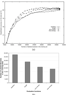
Figure 7

PLTIG parser: (a) A comparison of the evaluation functions’ learning curves. (b) A comparison of the evaluation functions for a test performance score of 80%.

Qualitatively comparing the learning curves in the figure, we see that with the ap-propriate evaluation function, sample selection does reduce the amount of annotation. Similarly to our findings in the PP-attachment study, the simple problem-space-based evaluation function, flen, offers only little savings; its performance is nearly

indistin-guishable from that of the baseline, for the most part.11 _{The evaluation functions based} on hypothesis performances, on the other hand, do reduce the amount of annotation in the training data. Of the two that we proposed for this category, the tree entropy eval-uation function,func, has a slight edge over the error-driven evaluation function,ferr.

For a quantitative comparison, let us consider the set of grammars that achieve an average parsing accuracy of 80% on the test sentences. We consider a grammar to be comparable to that of the baseline if its mean test score is at least as high as that of the baseline and if the difference between the means is not statistically significant. The baseline case requires an average of about 38,000 brackets in the training data. In contrast, to induce a grammar that reaches the same 80% parsing accuracy with the examples selected by func, the learner requires, on average, 19,000 training brackets.

Although the learning rate of ferr is slower than that of func overall, it seems to have

caught up in the end; it needs 21,000 training brackets, slightly more thanfunc. While

the simplistic sentence length evaluation function,flen, is less helpful, its learning rate

still improves slightly faster than that of the baseline. A grammar of comparable quality can be induced from a set of training examples selected byflen containing an average

of 28,000 brackets.12

4.2.2 A History-Based Learner. In the second experiment, the basic learning model is Collins’s (1997) Model 2 parser, which uses a history-based learning algorithm that takes statistics directly over the treebank. As a fully supervised algorithm, it does not have to iteratively reestimate its parameters and is computationally efficient enough for us to carry out a large-scale experiment. For this set of studies, the unlabeled candidate pool consists of around 39,000 sentences. The initial model is trained on 500 labeled seed sentences, and at each selection iteration, an additional 100 sentences are moved from the unlabeled pool into the training set. The parsing performance on the test sentences is measured in terms of the parser’s F-score, the harmonic average of the labeled precision and labeled recall rates over the constituents (Van Rijsbergen 1979).13

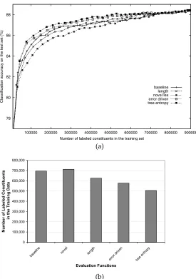
We plot the comparisons between different evaluation functions and the baseline for the history-based parser in Figure 8. The examples selected by the problem-space-based functions do not seem to be helpful. Their learning curves are, for the most part, slightly worse than the baseline. In contrast, the parsers trained on data selected by the error-driven and uncertainty-based functions learn faster than the baseline; and as before,func performs slightly better thanferr.

For the final parsing performance of 88%, the parser requires a baseline training set of 30,500 sentences annotated with about 695,000 constituents. The same performance can be achieved with a training set of 20,500 sentences selected byferr, which contains

about 577,000 annotated constituents; or with a training set of 17,500 sentences selected byfunc, which contains about 505,000 annotated constituents, reducing the number of

annotated constituents by 27%. Comparing the outcome of this experiment with that of

11 In this experiment, we have omitted the evaluation function for selecting novel lexical relationships,

flex, because the grammar does not use actual lexical anchors.

12 In terms of the number of sentences, the baselinefrandselected 2,600 sentences;flenselected 1,300 sentences; andferrandfunceach selected 900 sentences.

78 80 82 84 86 88

100000 200000 300000 400000 500000 600000 700000 800000 900000

Classification accuracy on the test set (%)

Number of labeled constituents in the training set

baseline length novel lex error driven tree entropy

(a)

0 100,000 200,000 300,000 400,000 500,000 600,000 700,000 800,000

base line

nove l

leng th

error d riven

tree entrop

y

Evaluation Functions

Number of Labeled Constituents

in the Training Data

(b)

Figure 8

Model 2 parser: (a) A comparison of the learning curves of the evaluation functions. (b) A comparison of all the evaluation functions at the test performance level of 88%.

the experiment involving the EM-based learner, we see that the training data reduction rates are less dramatic than before. This may be because bothfuncandferrignore lexical

items and chase after sentences containing words that rarely occur. Recent work by Tang, Luo, and Roukos (2002) suggests that a hybrid approach that combines features of the problem space and the uncertainty of the parser may result in better performance for lexicalized parsers.

5. Related Work

applications. Some examples include text categorization (Lewis and Catlett 1994), base noun phrase chunking (Ngai and Yarowsky 2000), part-of-speech tagging (Engelson Dagan 1996), spelling confusion set disambiguation (Banko and Brill 2001), and word sense disambiguation (Fujii et al. 1998).

More challenging are learning problems whose objective is not classification, but generation of complex structures. One example in this direction is applying sample selection to semantic parsing (Thompson, Califf, and Mooney 1999), in which sentences are paired with their semantic representation using a deterministic shift-reduce parser. A recent effort that focuses on statistical syntactic parsing is the work by Tang, Lou, and Roukos (2002). Their results suggest that the number of training examples can be further reduced by using a hybrid evaluation function that combines a hypothesis-performance-based metric such as tree entropy (“word entropy” in their terminology) with a problem-space-based metric such as sentence clusters.

Aside from active learning, researchers have applied other learning techniques to combat the annotation bottleneck problem in parsing. For example, Henderson and Brill (2002) consider the case in which acquiring additional human-annotated training data is not possible. They show that parser performance can be improved by using boosting and bagging techniques with multiple parsers. This approach assumes that there are enough existing labeled data to train the individual parsers. Another technique for making better use of unlabeled data is cotraining (Blum and Mitchell 1998), in which two sufficiently different learners help each other learn by labeling training data for one another. The work of Sarkar (2001) and Steedman, Osborne, et al. (2003) suggests that co-training can be helpful for statistical parsing. Pierce and Cardie (2001) have shown, in the context of base noun identification, that combining sample selection and cotraining can be an effective learning framework for large-scale training. Similar approaches are being explored for parsing (Steedman, Hwa, et al. 2003; Hwa et al. 2003).

6. Conclusion

In this article, we have argued that sample selection is a powerful learning technique for reducing the amount of human-labeled training data. Our empirical studies suggest that sample selection is helpful not only for binary classification tasks such as PP-attachment, but also for applications that generate complex outputs such as syntactic parsing.

We have proposed several criteria for predicting the training utility of the unla-beled candidates and developed evaluation functions to rank them. We have conducted experiments to compare the functions’ ability to select the most helpful training exam-ples. We have found that the uncertainty criterion is a good predictor that consistently finds helpful examples. In our experiments, evaluation functions that factor in the uncertainty criterion consistently outperform the baseline of random selection across different tasks and learning algorithms. For learning a PP-attachment model, the most helpful evaluation function is a hybrid that factors in the prediction performance of the hypothesis and the confidence for the values of the parameters of the hypothesis. For training a parser, we found that uncertainty-based evaluation functions that use tree entropy were the most helpful for both the EM-based learner and the history-based learner.

how-ever, hypothesis-parameter-based functions may be feasible under a multilearner set-ting, using parallel machines. Second, while in this work we focused on selecting entire sentences as training examples, we believe that further reduction in the amount of annotated training data might be possible if the system could ask the annotators more-specific questions. For example, if the learner is unsure only of a local decision within a sentence (such as a PP-attachment ambiguity), the annotator should not have to label the entire sentence.

In order to allow for finer-grained interactions between the system and the an-notators, we have to address some new challenges. To begin with, we must weigh in other factors in addition to the amount of annotations. For instance, the learner may ask about multiple substrings in one sentence. Even if the total number of la-bels were fewer, the same sentence would still need to be mentally processed by the annotators multiple times. This situation is particularly problematic when there are very few annotators, as it becomes much more likely that a person will encounter the same sentence many times. Moreover, we must ensure that the questions asked by the learner are well-formed. If the learner were simply to present the annotator with some substring that it could not process, the substring might not form a proper linguistic constituent for the annotator to label. Additionally, we are interested in exploring the interaction between sample selection and other semisupervised approaches such as boosting, reranking, and cotraining. Finally, based on our experience with parsing, we believe that active-learning techniques may be applicable to other tasks that produce complex outputs such as machine translation.

Appendix: Efficient Computation of Tree Entropy

As discussed in Section 4.1.2, for learning tasks such as parsing, the number of possi-ble classifications is so large that it may not be computationally efficient to calculate the degree of uncertainty using the tree entropy definition. In the equation for the tree entropy ofw(TE(w,G))presented in Section 4.1.2, the computation requires summing over all possible parses, but the number of possible parses for a sentence grows ex-ponentially with respect to the sentence length. In this appendix, we show that tree entropy can be efficiently computed using dynamic programming.

For illustrative purposes, we describe the computation process using a PCFG ex-pressed in Chomsky normal form.14 _{The basic idea is to compose the tree entropy of} the entire sentence from the tree entropy of the subtrees. The process is similar to that for computing the probability of the entire sentence from the probabilities of sub-strings (called Inside Probabilities). We follow the notation convention of Lari and Young (1990).

The inside probability of a nonterminal X generating the substring wi. . .wj is denoted ase(X,i,j); it is the sum of the probabilities of all possible subtrees that have X as the root and wi. . .wj as the leaf nodes. We define a new function h(X,i,j) to represent the corresponding entropy for the substring:

h(X,i,j) =− x∈X⇒∗wi...wj

P(x|G)lg(P(x|G))

where G is the current model. Under this notation, the tree entropy of a sentence, v∈VP

(v|G)lgP(v|G), is denoted ash(S, 1,n).

Analogously to the computation of inside probabilities, we compute h(X,i,j) re-cursively. The base case is when the nonterminalXgenerates a single token substring wi. The only possible tree hasXat the root, immediately dominating the leaf nodewi. Therefore, the tree entropy is

h(X,i,i) =e(X,i,i)lg(e(X,i,i))

For the general case,h(X,i,j), we must find all rules of the formX→YZ, whereYand Zare nonterminals, that have contributed towardX⇒∗ wi. . .wj. To do so, we consider all possible ways dividing up wi. . .wj into two pieces such that Y ⇒∗ wi. . .wk and

Z⇒∗ wk+1. . .wj:

h(X,i,j) =

j−1

k=i

(X→YZ)

hY,Z,k(X,i,j)

The functionhY,Z,k(X,i,j)is a portion ofh(X,i,j)that accounts for those parses in which the ruleX→YZis used and the division point is at wordwk. The nonterminalsYand Zmay, in turn, generate their substrings with multiple parses. LetY represent the set of parses for Y⇒∗ wi. . .wk; letZ represent the set of parses for Z⇒∗ wk+1. . .wj; and let xrepresent the parse step ofX→YZ. Then, there are a total ofY × Zparses, and the probability of each parse isP(x)P(y)P(z), wherey∈ Yandz∈ Z. To compute hY,Z,k, we need to sum over all possible parses:

hY,Z,k(X,i,j) = −

y∈Y,z∈Z

P(x)P(y)P(z)lg(P(x)P(y)P(z))

= −

y∈Y,z∈Z

P(x)P(y)P(z)(lgP(x) +lgP(y) +lgP(z))

= −P(x)lg(P(x))e(Y,i,k)e(Z,k+1,j) +P(x)h(Y,i,k)e(Z,k+1,j) +P(x)e(Y,i,k)h(Z,k+1,j)

Thus, the tree entropy of the entire sentence can be recursively computed from the entropy values of the substrings.

Acknowledgments

We thank Joshua Goodman, Lillian Lee, Wheeler Ruml, and Stuart Shieber for helpful discussions, and Ric Crabbe, Philip Resnik, and the reviewers for their constructive comments on this article. Portions of this work have appeared previously (Hwa 2000, 2001b); we thank the reviewers of those papers for their helpful comments. Parts of this work was carried out while the author was a graduate student at Harvard University, supported by the National Science Foundation under Grant No. IRI 9712068. The work is also supported by the Department of Defense contract RD-02-5700, and ONR MURI Contract FCPO.810548265.

References

Banko, Michele and Eric Brill. 2001. Scaling to very very large corpora for natural

language disambiguation. InProceedings of

the 39th Annual Meeting of the Association for Computational Linguistics, Toulouse, France, pages 26–33.

Blum, Avrim and Tom Mitchell. 1998. Combining labeled and unlabeled data

with co-training. InProceedings of the 1998

Conference on Computational Learning Theory, pages 92–100, Madison, WI. Brill, Eric and Philip S. Resnik. 1994. A rule

based approach to PP attachment

disambiguation. InProceedings of the 15th

Charniak, Eugene. 2000. A

maximum-entropy-inspired parser. In Proceedings of the First Meeting of the North American Association for Computational Linguistics, Seattle.

Cohn, David, Les Atlas, and Richard Ladner. 1994. Improving generalization

with active learning.Machine Learning,

15(2):201–221.

Collins, Michael. 1997. Three generative, lexicalised models for statistical parsing.

InProceedings of the 35th Annual Meeting of

the Association for Computational Linguistics, pages 16–23, Madrid.

Collins, Michael. 1999.Head-Driven Statistical

Models for Natural Language Parsing. Ph.D. thesis, University of Pennsylvania, Philadelphia.

Collins, Michael and James Brooks. 1995. Prepositional phrase attachment through

a backed-off model. InProceedings of the

Third Workshop on Very Large Corpora, Cambridge, MA, pages 27–38. Cover, Thomas M. and Joy A. Thomas.

1991.Elements of Information Theory. John

Wiley, New York.

Engelson, Sean P. and Ido Dagan. 1996. Minimizing manual annotation cost in supervised training from corpora. In Proceedings of the 34th Annual Meeting of the Association for Computational Linguistics, Santa Cruz, CA, pages 319–326. Freund, Yoav, H. Sebastian Seung, Eli

Shamir, and Naftali Tishby. 1997. Selective sampling using the query by committee

algorithm.Machine Learning,

28(2–3):133–168.

Fujii, Atsushi, Kentaro Inui, Takenobu Tokunaga, and Hozumi Tanaka. 1998. Selective sampling for example-based

word sense disambiguation.Computational

Linguistics, 24(4):573–598.

Henderson, John C. and Eric Brill. 2000. Bagging and boosting a treebank parser.

InProceedings of the First Meeting of the

North American Association for Computational Linguistics, Seattle, pages 34–41.

Hwa, Rebecca. 1998. An empirical

evaluation of probabilistic lexicalized tree

insertion grammars. InProceedings of the

36th Annual Meeting of the Association for Computational Linguistics and 17th International Conference on Computational Linguistics, Montreal, volume 1, pages 557–563.

Hwa, Rebecca. 2000. Sample selection for statistical grammar induction. In

Proceedings of 2000 Joint SIGDAT Conference on Empirical Methods in Natural Language Processing and Very Large Corpora, pages 45–52, Hong Kong, October.

Hwa, Rebecca. 2001a.Learning Probabilistic

Lexicalized Grammars for Natural Language Processing. Ph.D. thesis, Harvard University, Cambridge, MA. Hwa, Rebecca. 2001b. On minimizing

training corpus for parser acquisition. In Proceedings of the ACL 2001 Workshop on Computational Natural Language Learning (ConLL-2001), Toulouse, France, pages 84–89.

Hwa, Rebecca, Miles Osborne, Anoop Sarkar, and Mark Steedman. 2003. Corrected co-training for statistical

parsers. InProceedings of the ICML

Workshop on the Continuum from Labeled to Unlabeled Data in Machine Learning and Data Mining at the 20th International Conference of Machine Learning (ICML-2003),

Washington, DC, pages 95–102, August. Joshi, Aravind K., Leon S. Levy, and

Masako Takahashi. 1975. Tree adjunction

grammars.Journal of Computer and System

Sciences, 10(1): 136–163.

Lari, Karim A. and Steve J. Young. 1990. The estimation of stochastic context-free grammars using the inside-outside

algorithm.Computer Speech and Language,

4:35–56.

Larsen, Richard J. and Morris L. Marx. 1986. An Introduction to Mathematical Statistics and Its Applications. Prentice-Hall, Englewood Cliffs, NJ.

Lewis, David D. and Jason Catlett. 1994. Heterogeneous uncertainty sampling for

supervised learning. InProceedings of the

Eleventh International Conference on Machine Learning, San Francisco, pages 148–156.

Magerman, David. 1994.Natural Language

Parsing as Statistical Pattern Recognition. Ph.D. thesis, Stanford University, Stanford, CA.

Marcus, Mitchell, Beatrice Santorini, and Mary Ann Marcinkiewicz. 1993. Building a large annotated corpus of English: The

Penn Treebank.Computational Linguistics,

19(2):313–330.

Ngai, Grace and David Yarowsky. 2000. Rule writing or annotation: Cost-efficient resource usage for base noun phrase

chunking. InProceedings of the 38th Annual

Meeting of the Association for Computational Linguistics, pages 117–125, Hong Kong, October.

Pereira, Fernando C. N. and Yves Schabes. 1992. Inside-outside reestimation from

partially bracketed corpora. InProceedings

Pierce, David and Claire Cardie. 2001. Limitations of co-training for natural language learning from large datasets. In Proceedings of the 2001 Conference on Empirical Methods in Natural Language Processing (EMNLP-2001), pages 1–9, Pittsburgh, PA.

Ratnaparkhi, Adwait. 1998. Statistical models for unsupervised prepositional

phrase attachment. InProceedings of the

36th Annual Meeting of the Association for Computational Linguistics and 17th International Conference on Computational Linguistics, Montreal, volume 2, pages 1079–1085.

Sarkar, Anoop. 2001. Applying co-training methods to statistical parsing. In Proceedings of the Second Meeting of the North American Association for Computational Linguistics, Pittsburgh, pages 175–182, June.

Schabes, Yves and Richard Waters. 1993. Stochastic lexicalized context-free

grammar. InProceedings of the Third

International Workshop on Parsing Technologies, Tilburg, The Netherlands, and Durbuy, Belgium, pages 257–266. Steedman, Mark, Rebecca Hwa, Stephen

Clark, Miles Osborne, Anoop Sarkar, Julia Hockenmaier, Paul Ruhlen, Steven Baker, and Jeremiah Crim. 2003. Example

selection for bootstrapping statistical

parsers. InProceedings of the Joint

Conference of Human Language Technologies and the Annual Meeting of the North American Chapter of the Association for Computational Linguistics, Edmonton, Alberta, Canada, pages 236–243. Steedman, Mark, Miles Osborne, Anoop

Sarkar, Stephen Clark, Rebecca Hwa, Julia Hockenmaier, Paul Ruhlen, Steven Baker, and Jeremiah Crim. 2003. Bootstrapping statistical parsers from small datasets. In Proceedings of the Tenth Conference of the European Chapter of the Association for Computational Linguistics, Budapest, pages 331–338.

Tang, Min, Xiaoqiang Luo, and Salim Roukos. 2002. Active learning for statistical natural language parsing. In Proceedings of the 40th Annual Meeting of the Association for Computational Linguistics, Philadelphia, pages 120–127, July. Thompson, Cynthia A., Mary Elaine Califf,

and Raymond J. Mooney. 1999. Active learning for natural language parsing and

information extraction. InProceedings of

the Sixteenth International Conference on Machine Learning (ICML-99), pages 406–414, Bled, Slovenia.

Van Rijsbergen, Cornelis J. 1979.Information