Online Full Text

Abstract— This paper explores how the workload affects the efficiency of a production line. The line has partially cross-trained workers and the worksharing is organized under Dynamic Line Balancing (DLB) mechanism. Under this mechanism, the workers can help each other with some tasks, called shared tasks. To determine when to work on or pass the shared tasks to the next buffer, a heuristic rule called SRNS (Small R No Starvation) is used. Different configurations of workload are investigated. A measure of workload is proposed to ease the comparison. The results of simulating two-station line show the remarkable influence of workload on the efficiency and we find out its patterns as work-in-process WIP level changes. Also efficiency’s patterns with different shared task’ sizes are distinct for one configuration of workload to other configurations.

A.Index Terms—Dynamic Line Balancing, Workload, Worksharing, Simulation

I. INTRODUCTION

HE trend to producing variety of products with small quantities, reducing the WIP that is necessary to achieve the targeted throughput, increasing the utilization has magnified the importance of the cross-training. Actually, the original existence of this concept is in the cell manufacturing which is one of JIT revolution‟s outcomes.

The highest performance in these manufacturing environments can be achieved as much as workers approach to be full cross-trained. Moreover, the inventory is considered an absolute evil which represents the Japanese perspective and their strategy is to eliminate all factors that necessitate the inventory. Whereas, in western production systems it is a necessary evil as it makes production run smoothly [1]. Practically, having fully cross-trained workers is expensive since it will consume time and money. Additionally, the fast change of products will keep the need to continue training in high expenses, and on the other hand,

Manuscript received December 05, 2012; revised December 22, 2012 S. Kasmo is with the Industrial Engineering and Management Department, Tokyo Institute of Technology, 2-12-1 Oh-okayama, Meguro-ku, Tokyo 152-8552 Japan (phone: +81(80)-3310-2648; e-mail: kasmo.s.aa@ m.titech.ac.jp).

T. Enkawa is with the Industrial Engineering and Management Department, Tokyo Institute of Technology, (e-mail: [email protected]).

S. Suzuki is with the Industrial Engineering and Management Department, Tokyo Institute of Technology, (e-mail: Suzuki.s.ag@ m.titech.ac.jp).

the worker‟ speed will be slower with many tasks (full cross-trained) than that with limited number of tasks (partially cross-trained). Among different ways of applying worksharing, it is focused in this research on the way with partially cross-training of the workforce that it is referred to as Dynamic Line Balancing (DLB).

In DLB, introduced by Ostolaza et al. [2], the workers will stay in their stations; there is no movement between stations. Each worker is assigned to fixed tasks of a job which can be done only by him and can help the upstream and downstream workers in shared tasks after finishing the fixed ones. A worker chooses to pass on a job with the shared task undone or complete the shared task practically according to threshold rules depending on system information.

Moreover, there is buffer between stations which has two purposes as Ostolaza el al. [2] emphasized, providing work for the downstream station and providing storage for the upstream station. Their study show that by using DLB with a half-full buffer (HFB) control rule, the Work-In-Process (WIP) inventory can be reduced and the efficiency can be improved. McClain et al. [3] found that DLB can increase the efficiency even with no buffer. They used a new model called subtask model where the tasks of a job are divided into k subtasks and they employed Erlang-k distribution to represents the task times.

Two types of models (in term of information used to make a decision of passing or working on the shared task) have appeared in the literature; model A (as in [2]) and model B (as in [3]). In model A, the decision is supported by the workcontent in the downstream buffer only while in model B it is supported by the workcontent available to the downstream station which includes the one in the buffer and in the downstream station under processing not completed. Chen and Askin [4] proposed a new control rule with the model A which is called SRNS (Small R No Starvation). It is employed here as a control rule in our study. They show that this rule performs well by comparing its resulting performance with the optimal performance. They also compared in the other paper [5] between models A andB, and also between SRNS and HFB.

Gel et al. [6] compared between HFB and 50-50 rule which utilizes the ratio of workcontent at the upstream station to total workload in the system. They also study three factors that have notable influence on the worksharing. These factors are preemptability of shared task, granularity

A Study of the Effect of Workload on the

Performance of Production Lines under DLB

Mechanism

Salah Kasmo, Takao Enkawa, and Sadami Suzuki

of shared task, and processing time variability.

In this paper, we study a new factor which is the workload. The workload means here the sizes of fixed tasks of adjacent stations. Chen and Askin [5] demonstrated by using some examples how DLB can remedy the lost in the efficiency due to imbalanced fixed tasks. Also Gel et al. [6] treated this factor so briefly by one example and they found that the performance gets bad comparing with the balanced fixed workload. They also used the workload to compare between HFB and 50-50 rules. We study the workload in a totally different way. Cesani and Steudel [7] studied a pinion cell with two and three workers. Their results show that the workload assigned to the individual worker and the level of shared workload are significant factors determining the performance.

The objective of this research is to investigate the workload„s influence in DLB environment on the efficiency and find out its pattern through different workload configurations. This factor has not been addressed in a full picture before and if it is mentioned, it is briefly. In the previous researches, the balanced workload is mostly focused on which is a special case. However, the real production environments could encounter a variety of workload configurations. Here, several configurations are examined with different shared task‟ sizes. An easy to apply control rule is used (SRNS). A new measure of workload is proposed that facilitate tackling the objective.

The remaining of the paper is organized as follows section 2 explains the modeling assumptions, describes the control rule SRNS, and the workload measure is clarified. Section 3 gives simulation results and analysis. The last section summarizes the outcomes.

II.PROBLEM DESCRIPTION

A.Modeling Assumption

A two-station production line is considered. One worker is in each station. Worker 1 W1 attends at station 1 and worker 2 W2 attends at station 2. The buffer capacity is infinite, but the total number of jobs in the line is restricted to N number of jobs. This inventory level is reserved by the CONWIP discipline; Constant-Work-In-process. CONWIP, introduced by Spearman et al. [8], keeps Max WIP constant by preventing a new job to enter the line until a finished job leaves when the number of jobs reaches to Max WIP level. Since the goal is exploring the worksharing effect and since the high level of WIP in the line will hide the worksharing influence plus the resulting long cycle time and other side consequences accompanying that, the study is done with small numbers of N, 3, 4, 5.

Each job has three types of tasks, A, B, C. Task A can only be performed by W1 at station1 and task C can only be performed by W2 at station2. Both of tasks A, C are called fixed task. Task B can be done by either worker at his own station and it is called shared task. We assume that the tooling/ parts are available at the stations to operate task B.

The subtask model is used. In this model [3], a job consists of T number of equal subtasks to be performed in sequence. For example, a 2-3-4 task division refers to two

subtasks to task A, three subtasks to task B, and four subtasks to task C. The subtasks times are identically distributed, for instance, if they are exponentially distributed, the task will be Erlang-k distributed where k represents the number of subtasks that compose the task.

The job is processed in first come first serve (FCFS) queue. The shared task B is non-preemptive task. When a worker starts processing the shared task, it can be released till it becomes completed. The line is unidirectional, if a job is sent to the downstream station, it cannot return to the previous station. The workers‟ speeds are equal and W1 is the one who decides to pass on or keep working on the shared task.

B.Threshold Heuristic Rule

The used mechanism to manage the worksharing here is dynamic line balancing. In DLB, worker W1 after finishing task A has to make a decision whether to pass on or continue processing task B. This decision considers the current state of the system. Appropriate decisions [5] will give more work to station 2 when it is more available or potentially so, or pass less work onto it when otherwise. In other words, it tries to reduce the starvation and the blockage with fewer buffers.

However, it is not easy to make the best decision for all cases since this process is state-dependent and complicated to compute and implement in reality [6]. Threshold rules are more practical, where the decision is made based on the comparison between the available downstream workload and a specific threshold called R. Many threshold rules are existed in the literature. The easiest to apply and near-optimal rule is SRNS rule. In SRNS [4], W1 will start or keep working on the shared task if R or more units of subtasks are available in the buffer before station two. And the W1 will pass the shared task if the subtasks in buffer are less than R. The threshold value R is given by (1), where N is the CONWIP level and tC (tB) is the number of subtasks for

task C (B):





(

1

)

)

2

(

)

2

(

,

,

)

2

(

,

)

2

(





















t

N

t

if

t

N

t

t

N

t

if

t

N

R

The logic that is based on in this rule, is explained in details in [4], [5].

C.Workload Measure

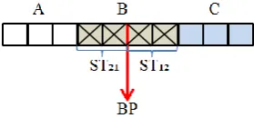
Workload refers here to the size of fixed task and their distribution between the stations. For example, a 3-4-3 task division has equal fixed task while 4-3-3 has different fixed task. 3-3-4 task division has the same shared task‟ size but the distribution of the fixed workload is opposite to the former division.

task division), the virtual breakeven point divides the job‟ subtasks into two equal groups of subtasks. The shared task consists of two subtasks from station 1‟ side and two subtasks from the other side. ST21 (ST12) represents the size

of shared task that can be done by worker 2(1) form station 1 (2)‟ side.

Fig. 1. The workload measure (two-station line) The measure of workload αij is defined by the ratio of the

shared subtasks‟ size done by worker (i) from station (j) side

to the total shared task‟ size as if all subtasks are distributed equally between two adjacent workers. The measure is given as follows;

)

2

(

/

B

ST





)

3

(

j

i

ST

ST

B





Taking 3-3-4 as an example, we have; B=3, ST12 =1, ST21 =2 and α12 =1/3, α21=2/3.

In this research, to explore several cases and get the more general results, ST12, ST12 each are given five values; 0, 1, 2,

3, 4. So we get 25 cases (as in Table I) that include also α12, α21 for each combination of ST12, ST12.

TABLE I

The Studied Combinations of ST12, ST12

A B C ST12 ST21 α12 α21

5 0 5 0 0 - -

4 1 5 0 1 0 1

3 2 5 0 2 0 1

2 3 5 0 3 0 1

1 4 5 0 4 0 1

5 1 4 1 0 1 0

4 2 4 1 1 0.5 0.5

3 3 4 1 2 0.33 0.67

2 4 4 1 3 0.25 0.75

1 5 4 1 4 0.2 0.8

5 2 3 2 0 1 0

4 3 3 2 1 0.67 0.33

3 4 3 2 2 0.5 0.5

2 5 3 2 3 0.4 0.6

1 6 3 2 4 0.33 0.67

5 3 2 3 0 1 0

4 4 2 3 1 0.75 0.25

3 5 2 3 2 0.6 0.4

2 6 2 3 3 0.5 0.5

1 7 2 3 4 0.4286 0.5714

5 4 1 4 0 1 0

4 5 1 4 1 0.8 0.2

3 6 1 4 2 0.67 0.33

2 7 1 4 3 0.5714 0.4286

1 8 1 4 4 0.5 0.5

III. SIMULATION RESULTS AND ANALYSIS

Visual Slam language (A simulation language) through AweSim software [9] is used to model and execute the

The total processing time of the job is 10 time unit (minutes) plus the variability. The processing time of a subtask is exponentially distributed with mean one, and then a task is Erlang-k where k is equal to the number of subtasks composing this task.

The efficiency is considered as a measure to evaluate the performance. It is defined as the ratio of simulated throughput rate over maximum achievable with balanced line, and deterministic processing times.

We combined the cases of study by considering the average efficiency in five combinations; (α12=0, α21=1),

(α12=1, α21=0), (α12=α21=0. 5), (α12=0.25, α21=0.75),

(α12=0.75, α21=0.25).The simulation results show that the

case without worksharing (5-0-5) has closer performance to the combination with worksharing that has the lowest efficiency among the others under all WIP levels.

The average results of efficiency for all other combinations show three distinguished patterns according to the WIP level in the line. The first, when N=3. Fig.2 presents the results. The plot shows that as α12 increases the

efficiency increases till it reaches the value 0.75 then decreases. α21 has an inversed pattern since α12+ α21 =1.

Where it increases till 0.25 then starts decreasing. The highest efficiency is achieved for (α12=0.75, α21=0.25) while

the lowest efficiency is achieved for (α12=0, α21=1). For

example, 4-4-2 has higher efficiency than 1-4-5.

Fig. 2. The change of efficiency with α under N=3 By comparing between (α12=0, α21=1), (α12=1, α21=0), we

find that the second combination presents higher efficiency. The same is for (α12=0.25, α21=0.75), (α12=0.75, α21=0.25),

but with better performance than the previous. The reason might be that when α12 is 0 or small, it means a large fixed

task for station 2. As a result, this large fixed task will cause a smaller throughput since station 2 becomes bottleneck. This could be alleviated as the fixed task of station 2 get smaller or in other word as α12 becomes bigger. However,

this amount of fixed task or α12 has a limit which is 0.75

after that the effect gets inversed as station 1 will be the bottleneck. Beside to the above reason, the small number of WIP in the line deepens this difference, since the station one could starve. Another observation is when α12=α21=0. 5, the

efficiency is between (α12=0.25, α21=0.75), (α12=0.75, α21=0.25). Let‟s take an example to make the previous

discussion clearer. Fig.3 represents the different

combinations of α under B=3.

The second case when N=4. Here as in Fig.4, the differences between the opposite combinations get smaller. (α12=0.25, α21=0.75), (α12=0.75, α21=0.25) have small

difference and also for (α12=0, α21=1), (α12=1, α21=0).

However, the other results are same except for α12=α21=0. 5

which becomes as same as (α12=0.75, α21=0.25). Here, the

surplus of WIP in the line moderates the starvation of station one which results to minimize the differences between the opposite combinations.

Fig. 3. Efficiency with different task divisions and B=3

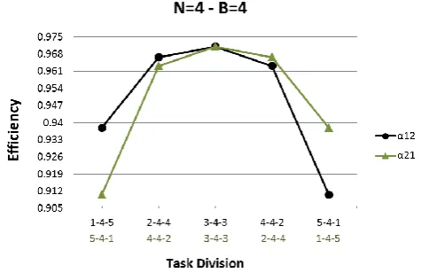
Fig. 4. The change of efficiency with α under N=4 For example, with B=4, we get Fig.5 which demonstrates the pattern of workload when N increases to 4.

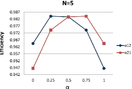
The last case when N equals to 5. The pattern is opposite to the first case and the differences between the opposite combinations are less. As in Fig.6, the efficiency get better as α12 get bigger then decreases after 0.5 while α21 continues

improving the efficiency till 0.75. The combination (α12=0, α21=1) presents higher efficiency than (α12=1, α21=0). Also

the combination (α12=0.25, α21=0.75) has better efficiency

than (α12=0.75, α21=0.25) which is opposite to the case with N=3. (α12=0.25, α21=0.75) gives the highest efficiency and α12=α21=0. 5 also has the same efficiency.

When α12=1, that means the fixed task of station 1 gets so

big (in this study 5), in other words it becomes a bottleneck. That will prevent inserting more jobs into the line resulting starvation in the station 2. On other hand, when α12=0, which

means the station 2 gets a bottleneck. Here, no station will starve since there is a surplus of WIP. For α12=0.25, 0.75,

the same analysis can be considered and because α12 is

between 0 and 1 so that gives better performance since it will reduce the effect of bottleneck. Fig.7 presents the same pattern as discussed before with B=5.

Fig. 6. The change of efficiency with α under N=5

Fig. 7. Efficiency with different task divisions and B=5 We noticed some differences between the examples and the average patterns and the reason is that the efficiency is also affected by the size of the shared task. Fig.8 plots the efficiency with different shared task‟ size which is represented by fraction of shared task to total work (β) and under (α12=1, α21=0). The performance deteriorates as β

increases after 0.2. In this case, station 1 has a big fixed task and as shared task‟ size gets bigger, additional tasks will be available to W1. As a result, station 2 starves for long time. On the other side, there is no remarkable change with (α12=0, α21=1) as the size of shared task changes except (the plot is

not presented). The efficiency remains almost the same as β increases. Here, the station 2 will be the bottleneck, and since W1 who will decides to pass or keep the shared task, he can adapt with the bottleneck‟s effect by keeping working on the shared task more frequently.

Fig. 8. Efficiency versus β under α12=1, α21=0

The balanced fixed workload (Fig.9) which can be translated as α12=α21=0. 5 has the same trend as in previous

papers [3], [4], [5]. The performance improves as β increases till 0.4 then the efficiency declines.

Fig. 9. Efficiency versus β under α12=α21=0. 5

IV. CONCLUSION

A two-station production line run under DLB policy is simulated. We considered SRNS rule as a threshold rule to keep or pass the shared task. The number of jobs in the line is controlled by CONWIP procedure and small level of WIP is employed since the large one will hide the effect of worksharing. Several workload configurations with different sizes of shared task are investigated. We proposed a measure for workload to find out the pattern of efficiency with different configurations of workload.

REFERENCES

[1] S. Shingo, Non-stock production: the Shingo system for continuous improvement. Productive Press, 1985, pp.xx.

[2] J. Ostolaza, J. McClain, and J. Thomas, “The use of dynamic (state-dependent) assembly-line balancing to improve throughput,” Journal of Manufacturing and Operation Management, vol.3, pp.105-133, 1990.

[3] J.O. McClain, J. Thomas, and C. Sox, “On-the-fly line balancing with very little WIP,” International Journal of Production Economics, vol.27, pp. 283–289, 1992.

[4] J. Chen, and R.G. Askin, “Throughput maximization in serial production lines with worksharing,” International Journal of Production Economics, vol. 99, pp.88–101, 2006.

[5] R.G. Askin, and J. Chen, “Dynamic task assignment for throughput maximization with worksharing,” European Journal of Operational Research, vol.168, pp.853– 869, 2006.

[6] E. S. Gel, W. J. Hopp, and M. P. Van Oyen, “Factors affecting opportunity of worksharing as a dynamic line balancing Mechanism,” IIE Transactions, Vol.34, No.10, pp.847-863, 2002.

[7] V. I. Cesani, and H. J. Steudel, “A study of labor assignment flexibility in cellular manufacturing systems,” Computers and Industrial Engineering, Vol.48, pp. 571-591, 2005.

[8] M. L. Spearman, D. L. Woodruff, and W. J. Hopp, “CONWIP: A pull alternative to Kanban,” Production Planning and Control, Vol.28, No.5, pp.879-894, 1990.