An Approach to Classify Heritage Sites Architecture Using Convolution Neural Networks

An Approach to Classify Heritage Sites

Architecture Using Convolution Neural Networks

Manikantan. E1, Bhavana2. V, Niveditha S. Prasad3, Nandan. K4, Asha. R.N5

1, 2, 3, 4

Student, Global Academy of Technology

5

Asst. Prof., Dept. of CSE, Global Academy of Technology

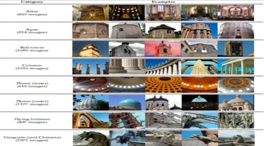
Abstract: In this project, we have explored the use of Convolution Neural Networks for semantic classification of heritage site architectures like dome, bell tower, glass, and gargoyle. We have tested our proposed system with two different learning modalities. Besides conventional training from scratch, we have resorted to pre-trained networks that have been fine-tuned on a huge amount of data in order to avoid overfitting problems and to reduce design/computing time. Experiments on a dataset we have built by ourselves from Heritage repository show that with the help of this step of fine-tuning, one of the simplest (and oldest) networks able to produce similar results than more sophisticated ones as ResNet which is pretty 3 times more consuming in computing time, mainly due to the number of the layer it uses. With this model, we have been able to show that our model can classify in the right way more than 98% of the images belonging to the dataset test. From now, this model can be used to classify the full dataset of the Heritage repository.

I. INTRODUCTION

From a couple of years, the project Heritage Observatory (HeObs) collects photos, post-cards and any graphical documents about South-East Asia. This collection comes from both private and public images. The huge amount of data, at this time more than

100,000 documents, is available through a websiteand any one concerns can freely annotate them. In order to present the dataset in a

friendlier user interface, a first step of automatic classification can be achieved to split the dataset following the semantic categories described usually in this domain: heritage site architecture. From this classification, the volunteers can chose the type of images they prefer to annotate. Even, this first classification is not very précised, this first step seems to be essential to begin the work.

Labeling an image according to a set of semantic categories is ordinary goal for image classification. Until now, this problem remains difficult to solve because of intra-class variability coming from different lighting conditions, misalignment, non-rigid deformations. Numerous efforts have been made to evaluate the intra-class variability by manually designing low-level features used for classification tasks. Although the low-level features can be hand crafted with great success for certain data and tasks, designing effective features for new data and tasks usually requires new domain knowledge because most hand-crafted features cannot simply be adapted to new conditions [1] [2]. Learning features from data of interest is considered as a plausible method of remedying the limitations of handcrafted features and at this time, using Convolutional Neural Networks (CNNs) to learn image features is one of the most popular methods. In this project, we have tested our system of CNNs to appreciate to provide the best results on our data set. To cope with the scarcity of training image dataset, we have explored various training modalities: not only the usual training from scratch but also the fine-tuning of pre-trained networks. Besides that, we have lead our own tuning on the CNNs parameter values to improve final results.

A. Deep Learning With Convolution Neura Network

Artificial neural networks initially take inspiration from models of the biological brain, and try to reproduce some of its functions by using simple but massively interconnected processing units, the neurons. A typical neural network architecture contains several layers of neurons feeding one another. Deep learning has provided excellent results in object recognition, image classification and retrieval.

Figure 1: Visualization of first filters from Krizhevsky example

In current CNNs, each layer comprises various sublayers of neurons operating in parallel on the previous layer, so as to extract a number of features at once, like a bank of filter does. Krizhevsky et al. give an example ([3]) of filters learned in the first layer of a CNN designed for image classification (see Fig.1). Each filter elaborates the three input color bands, producing by convolution a corresponding feature map. In this example, 96 feature maps are produced as output of the second layer, which become the input of the next one.

Figure 2: Generic CNN architecture

CNNs have been introduced many years ago but become popular more recently. In one hand, the fast growth of affordable computing power, especially graphical processing units (GPUs), and the diffusion of large datasets of labeled images for training have increased drastically the interest for this method. On the other hand, new researches have contributed to many innovative solutions for faster and more reliable learning. For example, the rectified linear unit (ReLU) [11], a neuron with a simplified non-linearity which allows much faster training, and techniques to reduce over-fitting, such as dropout [12], or data augmentation. The first CNN exploiting all these solutions, proposed in the seminal work of Krizhevsky et al. [3], improved image classification results by more than 10% with respect to the previous state of the art.

II. LITERATURE SURVEY

A. Manh-Tu VU, Marie Beurton-Aimar, and Van-Linh LE

B. K. He, X. Zhang, S. Ren, and J. Sun

Is proposed thatdeeper neural networks are more difficult to train. We present a residual learning framework to easy the training of

networks that are substantially deeper than those used. We explicitly reformulate the layers as learning the residuals functions with reference to the layer inputs, instead of learning and reference functions we provide comprehensive empirical evidence showing that these residuals networks are easier to optimize and can gain accuracy from considerably increased depth. On the ImageNet data set we evaluate residual nets with a deep of upto 152layers, 8x deeper than VGG nets but still having lower complexity. And ensemble of the residual nets achieves less error on the ImageNet test set.

C. M. Peng, C. Wang, T. Chen, and G. Liu

Near-infrared (NIR) face recognition has attracted increasing attention because of its advantage of illumination invariance. However, traditional face recognition methods based on NIR are designed for and tested in cooperative-user applications. In this

paper, we present a convolutional neural network (CNN) for NIR face recognition (specifically face identification) in non

-cooperative-user applications. The proposed NIRFaceNet is modified from GoogLeNet, but has a more compact structure designed

specifically for the Chinese Academy of Sciences Institute of Automation (CASIA) NIR database and can achieve higher

identification rates with less training time and less processing time. The experimental results demonstrate that NIRFaceNet has an

overall advantage compared to other methods in the NIR face recognition domain when image blur and noise are present. The performance suggests that the proposed NIRFaceNet method may be more suitable for non-cooperative-user applications.

1) Existing System

a) Support vector machine algorithm is a supervised classification technique which is used in many of the image processing.

b) a linear SVM finds the hyper plane leaving the largest possible fraction of points of the same class on the same side.

c) In the existing system people collect the images to build the training set that is necessary in order for the test image to be compared.

d) To collect the picture of interest the user must visit those particular places, which is time consuming and most of the time it may

not be possible for the user to visit the places. Disadvantage

a) It consumes more time gives less accuracy.

2) Proposed System: In this work, we have used CNNs to carry out heritage image classification. Our architectures have been already proposed and tested in the literature, especially for computer vision tasks, and most of them have been implemented and made available online. In this work, we have focused on our architecture is made up of 5 conv layers, max-pooling layers,

dropout layers, and 3 fully connected layers. It designed for classification with 1000 possible categories.The overview of the

system design is that the user can uploads the heritage image to the system. The CNN classifier reshapes the images to set the neurons to understand the features of the images. Once the feature is identified the images is labeled to particular category and is stored into a folder.

III. MODULES

A. Feature Extraction

B. LBP Features

C. Training Image Set

1) Module 1

a) Module Name: Feature Extraction

b) Functionality: This function will extract the features of an image using Histogram of Oriented Gradients. c) Input: Images.

d) Output: Image processing basically to serve the purpose of object detection. e) Algorithm used: Histogram of oriented gradients.

2) Module 2

a) Module Name: LBP Features

b) Functionality: This function will labels the pixels of an image by thresholding the neighborhood of each pixel and considers the result as a binary number.

c) Input: Images.

d) Output: Texture classification and segmentation, image retrieval and surface inspection.

e) Algorithm used: Local binary pattern.

3) Module 3

a) Module Name: Training Image Set

b) Functionality: This function will holds vector information that is vital to the input. When the network gets trained, this feature vector is then further use for classification.

c) Input: Image Set.

d) Output: Extraction of Representations using Deep CNN to label the image to appropriate category. 4) Algorithms

a) Histogram Of Oriented Gradients

i) Step 1: Gradient Computation: The first step of calculation in many feature detectors in image pre-processing is to ensure

normalized color and gamma values. As Dalal and Triggs point out, however, this step can be omitted in HOG descriptor computation, as the ensuing descriptor normalization essentially achieves the same result. Image preprocessing thus provides little impact on performance. Instead, the first step of calculation is the computation of the gradient values. The most common Algorithm implementation method is to apply the 1-D centered, point discrete derivative mask in one or both of the horizontal and vertical directions. Specifically, this method requires filtering the color or intensity data of the image with the following filter kernels: Dalal and Triggs tested other, more complex masks, such as the 3x3 Sobel mask or diagonal masks, but these masks generally performed more poorly in detecting humans in images. They also experimented with Gaussian smoothing before applying the derivative mask, but similarly found that omission of any smoothing performed better in practice.

ii) Step 2: Orientation Binning: The second step of calculation is creating the cell histograms. Each pixel within the cell casts a

weighted vote for an orientation-based histogram channel based on the values found in the gradient computation. The cells themselves can either be rectangular or radial in shape, and the histogram channels are evenly spread over 0 to 180 degrees or 0 to 360 degrees, depending on whether the gradient is “unsigned” or “signed”. Dalal and Triggs found that unsigned gradients used in conjunction with 9 histogram channels performed best in their human detection experiments. As for the vote weight, pixel contribution can either be the gradient magnitude itself, or some function of the magnitude. In tests, the gradient magnitude itself generally produces the best results. Other options for the vote weight could include the square root or square of the gradient magnitude, or some clipped version of the magnitude.

iii) Step 3: Descriptor Blocks: To account for changes in illumination and contrast, the gradient strengths must be locally

with 9 histogram channels. Moreover, they found that some minor improvement in performance could be gained by applying a Gaussian spatial window within each block before tabulating histogram votes in order to weight pixels around the edge of the blocks less. The R-HOG blocks appear quite similar to the scale-invariant feature transform (SIFT) descriptors; however, despite their similar formation, R-HOG blocks are computed in dense grids at some single scale without orientation alignment, whereas SIFT descriptors are usually computed at sparse, scaleinvariant key image points and are rotated to align orientation. In addition, the R-HOG blocks are used in conjunction to encode spatial form information, while SIFT descriptors are used singly. Circular HOG blocks (C-HOG) can be found in two variants: those with a single, central cell and those with an angularly divided central cell. In addition, these C-HOG blocks can be described with four parameters: the number of angular and radial bins, the radius of the center bin, and the expansion factor for the radius of additional radial bins. Dalal and Triggs found that the two main variants provided equal performance, and that two radial bins with four angular bins, a center radius of 4 pixels, and an expansion factor of 2 provided the best performance in their experimentation(to achieve a good performance, at last use this configure). Also, Gaussian weighting provided no benefit when used in conjunction with the C-HOG blocks. C-HOG blocks appear similar to shape context descriptors, but differ strongly in that C-HOG blocks contain cells with several orientation channels, while shape contexts only make use of a single edge presence count in their formulation.

iv) Step 4: Block Normalization: Dalal and Triggs explored four different methods for block normalization. Let be the

non-normalized vector containing all histograms in a given block, be its k-norm for and be some small constant. L2-norm followed by clipping (limiting the maximum values of v to 0.2) and renormalizing, as in L1-norm: L1-sqrt: In addition, the scheme L2-hys can be computed by first taking the L2-norm, clipping the result, and then renormalizing. In their experiments, Dalal and Triggs found the L2-hys, L2-norm, and L1-sqrt schemes provide similar performance, while the L1-norm provides slightly less reliable performance; however, all four methods showed very significant improvement over the non-normalized data.

v) Step 5: Object Recognition: HOG descriptors may be used for object recognition by providing them as features to a machine

learning algorithm. Dalal and Triggs used HOG descriptors as features in a support vector machine (SVM) [9]; however, HOG descriptors are not tied to a specific machine learning algorithm.

5) Algorithm 2

a) Local binary patterns

i) Step 1: Divide the examined window into cells (e.g. 16x16 pixels for each cell).

ii) Step 2: For each pixel in a cell, compare the pixel to each of its 8 neighbors (on its left-top, left-middle, left-bottom, right-top, etc.). Follow the pixels along a circle, i.e. clockwise or counter-clockwise.

iii) Step 3: Where the center pixel's value is greater than the neighbor's value, write "0". Otherwise, write "1". This gives an 8-digit binary number (which is usually converted to decimal for convenience).

iv) Step 4: Compute the histogram, over the cell, of the frequency of each "number" occurring (i.e., each combination of which pixels are smaller and which are greater than the center). This histogram can be seen as a 256-dimensional feature vector. v) Step 5: Optionally normalize the histogram.

vi) Step 6: Concatenate (normalized) histograms of all cells. This gives a feature vector for the entire window. 6) Algorithm 3

a) Fully Connected Layer

i) Step 1: The neuron in the fully-connected layer detects a certain feature; say, a nose.

ii) Step 2: It preserves its value.

iii) Step 3: It communicates this value to both the “dog” and the “cat” classes.

iv) Step 4: Both classes check out the feature and decide whether it's relevant to them.

IV. RESULTS

The most important metrics we have considered were test accuracy and train accuracy because they show the classification quality. In the Table 1 reports synthetic results for the four heritage sites architectures and the two design approaches considered.

Architecture Test Accuracy Train Accuracy

Bell Tower 97.41 97.4

Dome 98.35 96.9

Gargoyle 98.58 95.52

Glass 98.82 97.39

Table 1: Classification accuracy (in percent) of proposed CNN-Based solutions.

The observation is that the fine-tuning approach provides the best results in all cases, as expected. Reaching an overall test accuracy of 97.41%, 98.35%, 98.58% and 98.82% with our proposed system, respectively. This is about 5%, 8%, 11% and 56% better, respectively, than the design from other architecture, confirming the interest of fine-tuning when training data are limited.

V. CONCLUSION

We have addressed the heritage site Architecture classification task by resorting to convolutional neural networks. Four promising architectures have been considered with two design modalities. Experiments on our dataset with several different point-of views have provided insightful information. As expected, training a CNN with fine-tuning, involving several layers of the architecture, provides the best results, in general. About comparison between CNN models.

REFERENCES

[1] A. Krizhevsky, I. Sutskever, and G. E. Hinton, “Imagenet classification with deep convolutional neural networks,” Commun. ACM, vol. 60, pp. 84–90, May 2017.

[2] C. Szegedy, W. Liu, Y. Jia, P. Sermanet, S. E. Reed, D. Anguelov, D. Erhan, V. Vanhoucke, and A. Rabinovich, “Going deeper with convolutions,” CoRR, vol. abs/1409.4842, 2014.

[3] K. He, X. Zhang, S. Ren, and J. Sun, “Deep residual learning for image recognition,” CoRR, vol. abs/1512.03385, 2015. [4] J. Hu, L. Shen, and G. Sun, “Squeeze-and-excitation networks,” CoRR, vol. abs/1709.01507, 2017.

[5] M. Castelluccio and al, “Land use classification in remote sensing images by convolutional neural networks,” CoRR, vol. abs/1508.00092, 2015. [6] Y. LeCun, Y. Bengio, and G. Hinton, “Deep learning,” Nature, vol. 521, pp. 436 EP –, 05 2015.

[7] C. Szegedy and al, “Rethinking the inception architecture for computer vision,” CoRR, vol. abs/1512.00567, 2015.

[8] M. Peng, C. Wang, T. Chen, and G. Liu, “Nirfacenet: A convolutional neural network for near-infrared face identification,” Information, vol. 7, no. 4, 2016. [9] G. E. Hinton, “Rectified linear units improve restricted boltzmann machines vinod nair,” International Conference on Machine Learning, 2010.

[10] G. E. Hinton and al, “Improving neural networks by preventing coadaptation of feature detectors,” CoRR, vol. abs/1207.0580, 2012.

[11] K. Chatfield, K. Simonyan, A. Vedaldi, and A. Zisserman, “Return of the devil in the details: Delving deep into convolutional nets,” CoRR, vol. abs/1405.3531, 2014.

[12] M. Lin, Q. Chen, and S. Yan, “Network in network,” CoRR, vol. abs/1312.4400, 2013.

[13] S. Arora, A. Bhaskara, R. Ge, and T. Ma, “Provable bounds for learning some deep representations,” CoRR, vol. abs/1310.6343, 2013. [14] K. He and J. Sun, “Convolutional neural networks at constrained time cost,” CoRR, vol. abs/1412.1710, 2014.