Improving the Real-Time Concurrent Constraint Calculus with a Delay Declaration

Improving the Real-Time Concurrent Constraint Calculus with a Delay

Declaration

Gerardo M. Sarria M.

Abstract—The Real-Time Concurrent Constraint Programming Calculus (rtcc) is a model of concur-rency developed to specify systems with real-time be-haviour. In this paper we enhance this calculus by extending the concept of time as a discrete sequence of minimal units that we will callticks. We also add a new construct tortccto be able of delaying the exe-cution of a process for an amount of ticks. The oper-ational semantics were adapted to support these new features. We argue that this extension makes the cal-culus temporally homogeneous and allows modeling real-time systems (such as an improvisation system where time is an inflexible notion) in a more precise way.

Keywords: process calculi, rtcc, operational semantics, delay declaration

1

Introduction

Thertcc calculus [11] is a ccp-based formalism [10], ex-tension of thentcc calculus [8]. rtcc is obtained from

ntccby adding a construct for specifying strong preemp-tion and by extending the transipreemp-tion system with sup-port for resources, limited time and true concurrency. This calculus allows modeling real-time and reactive be-haviour.

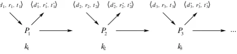
In reactive systems, time is conceptually divided into dis-crete intervals (ortime units). In a time interval, a pro-cess receives a stimulus from the environment, it com-putes (reacts) and responds to the environment. In the case of rtccthe stimulus is a tuple consisting of a con-straint representing the initial store, the available num-ber of resources and the duration of the time unit, and responds with another tuple consisting of a constraint representing the final store, the maximum number of re-sources used in calculations and the time spent in them. A reactive system is shown in figure 1. For eachPithere

is an stimulus⟨di, ri, ti⟩and a response ⟨d′i, r′i, t′i⟩ in the

time unitki.

To model real time, we assume that each time unit is a clock-cycle in which computations (internal transitions) involving addition of information to the store (tell op-erations) and querying the store (ask operations) take a

∗_{AVISPA Research Group. Pontificia Universidad Javeriana,}

Cali - Colombia. Email: [email protected]

1

k k2 k3

1

P P₂ P₃

r’

d’1, 1,t’1 d2,r2,t2 r1

1, ,t1 2,r’2,t’2 d3,r3,t3 d’3,r’3,t’3

... d’

d

Figure 1: Reactive System

particular amount of time dependent on the constraint system. A discrete global clock is introduced and it is assumed that this clock is synchronized with the physical time (i.e. two successive time units in this calculus cor-respond exactly to two moments in the physical time). We also assume that the environment provides the exact duration of the time unit. That is, processes may not have all the time they need to run, instead, if they do not reach their resting point in a particular time, some (or all) of their computations not done will be discarded before the time unit is over. The duration will be then the available time that processes have to execute. We will take this available time as a natural number; this allows to think of time as a discrete sequence of minimal units that we will callticks.

Thertcc calculus provides a way of executing unit de-lays and weak time-outs with the constructsnextP and

unlessc next P. We realized that just with these con-structs a calculus is not able to express neither strong time-outs [1]: “if an event A does not happen by time t, cause event B to happen at time t”, nor real delays within the current time unit.

ProcessnextPactivatesPthe next time unit. Then this construct delays a process an amount of time given by the environment (the duration of the time unit). This means that there is no total control over the exact duration of the retard and might be more than the time wanted. To eliminate this drawback, we will add the construct:

delayP forδ

The main contributions of this paper are: 1) the intro-duction tortccof a new construct to delay the execution of a process within a time unit, 2) an example illustrating the potential of the new feature, 3) an extension of the operational semantics to support the new construct, and 4) the explanation of some properties of processes.

2

The Calculus

Here we describe the enhanced syntax and the extended operational semantics forrtcc. We begin by introducing the notion of constraint system, very important in ccp-based calculi.

Constraint System. Thertcc processes are parame-terized in aconstraint system which specifies what kind of constraints handle the model. Formally, it is a pair (Σ,Δ) where Σ is a signature (a set of constants, func-tions and predicates) and Δ is a first order theory over Σ (a set of first-order sentences with at least one model).

Given a constraint system, the underlying language L of the constraint system is a tuple (Σ,V,S), where V is a set of variables, and S is a set with the symbols

¬,∧,∨,⇒,∃,∀ and the predicates true and false. A constraint is a first-order formulae constructed inL.

A constraintcentails a constraintdin Δ, notationc⊧_Δ d, iff c ⇒ dis true in all models of Δ. The entailment relation is written ⊧ instead of⊧_Δ if Δ can be inferred from the context.

For a constraint system D, the set of elements of the constraint system is denoted by∣D∣ and ∣D∣0 represents

its set of finite elements. The set of constraints in the underlying constraint system will be denoted byC. The conjunction of all posted constraints will be called the store.

Process Syntax. The Processes P, Q, . . . ∈ P roc are built from constraints c ∈ C and variables x ∈ V in the underlying constraint system by the following syntax:

P, Q, . . . ::= tell(c) ∣ ∑_i∈I whenci doPi∣ P∥Q

∣ localxin P ∣ unlesscnext P

∣ catch cin P finallyQ ∣ nextP

∣ delay P forδ ∣ !P ∣ ⋆P

Intuitively, the process tell(c) adds constraint c to the store within the current time unit. The ask processwhen

cdo P is generalized with a non-deterministic choice of the form _∑i∈I when ci do Pi (I is a finite set of

in-dices). This process, in the current time unit, must non-deterministically choose one of thePj(j∈I) whose

corre-sponding guard constraintcjis entailed by the store, and

execute it. The non-chosen processes are precluded. Two processes P and Q acting concurrently are denoted by the processP∥Q. In one time unitP and Qoperate in parallel, communicating through the store by telling and asking information. The “∥” operator is defined as left associative. The processlocalxinP declares a variable xprivate toP (hidden to other processes). This process behaves likeP, except that all information aboutx pro-duced byP can only be seen by P and the information aboutxproduced by other processes is hidden toP. The weak time-out process,unless cnext P, represents the activation ofP the next time unit ifc cannot be inferred from the store in the current time interval (i.e. d⊭c). Otherwise,Pwill be discarded. The strong time-out pro-cess,catchcinP finallyQ, represents the interruption ofP in the current time interval when the store can entail c; otherwise, the execution ofP continues. When process P is interrupted, process Qis executed. IfP finishes,Q is discarded.

The execution of a processP now can be delayed in two ways: with delay P for δ the process P is activated in the current time unit but at least δ ticks after the beginning of the time unit, whilst withnextP the pro-cess P will be activated in the next time interval. The operator “!” is used to define infinite behaviour. The process !P represents P ∥ next P ∥ next(next P) ∥ . . ., (i.e. !P executes P in the current time unit and it is replicated in the next time interval). An arbi-trary (but finite) delay is represented with the operator “⋆”. The process⋆P represents an unbounded but finite P + next P + next(next P) + . . ., (i.e. it allows to model asynchronous behaviour across the time intervals).

The guarded-choice summation process_∑i∈I whenc_ido

P_i is actually the abbreviation of

whenc_i1 doP_i1+. . .+whenc_in doP_in

whereI= {i1, . . . , in}. The symbol “+” is used for binary

summations (similar to the choice operator from CCS [6]). If there is no ambiguities, the “whenc do” can be omitted whenc=true, that is,∑_i∈IPi. The process that

do nothing isskip. The inactivity process is defined as the empty summation∑_i∈∅Pi. This process is similar to

process 0 of CCS and ST OP of CSP [5]. Furthermore, terminated processes will always behave like skip. We write_∏i∈IP_i, whereI= {i₁, . . . , i_n}to denote the parallel composition of all theP_i, that is,P_i1 ∥. . .∥P_in. When processQisskip, the “finallyQ” part in processcatch

c in P finally Q can be omitted, that is, we can write

catch c in P. A nest of delta delay processes such as

delay (delay P for δ₁) for δ₂ can be abbreviated to

delay P for δ1+δ2. Notation nextn P (where next

is repeatedntimes) is written to abbreviate the process

∏i∈InextiPand∑i∈InextiP, respectively. For example,

process !_[m,n]Pmeans thatPis always active between the nextmandm+ntime units.

Now we will show a simple example illustrating the specification of temporal behaviour in this calculus.

Example 2.1. Suppose a simple improvisation situation where there are two machines M1 and M2. The first

machineM₁performs a single random action from a list Actions every 15 ticks. The second machine M₂ must follow it, that is, perform a series of actions depending on the action performed by M₁. Additionally, in some occasions M₁ not only performs a single action but two in the same time unit (it performs one action and 5 ticks latter performs another). In this case M₂ must stop its performance and try to follow the second action (there may be cases in which this is not possible due to the limit of time). This behaviour can be modeled as follows:

First, we have to modelM1:

M₁def= ! ∑

i∈Actions

tell(action1=i) ∥

⋆ delay ∑

i∈Actions

tell(action2=i)for5

Now for the second machine we assume a process F ollowingActions that calculates the actions to follow and performs them. Also, we assume an action 0 ∉ Actions. ThusM2 is modeled:

M2def= ! whenaction1≠0 do

catch action2≠0

in F ollowingActions_(action1)

finallyF ollowingActions_(action2) To model the whole system we simply launch the process M1∥M2.

3

Operational Semantics

The operational semantics can be formally described by means of a transition system conformed by the set of processesP roc, the set of configurations Γ and transition relations→and ⇒. A configurationγ is a tuple⟨P, d, t⟩ whereP is a process,dis a constraint in C representing the store, andtis the amount of time left to the process to

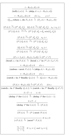
be executed. The transition relations → = {→⟨r⟩, r∈Z+} and⇒are the least relations satisfying the rules in tables 1 and 2.

Theinternal transition rule ⟨P, d, t⟩→ ⟨r P′, d′, t′⟩ means that in one internal time using r resources process P with store dand available time t reduces to process P′ with store d′ and leaves t′ time remaining. We write

Table 1: Internal Transition Rules of rtcc

t−Φ_T(c, d) ≥0

⟨tell(c), d, t⟩ → ⟨1 skip, d∧c, t−Φ_T(c, d)⟩

t−Φ_A(cj, d) ≥0 d⊧cj, j∈I

⟨∑i∈IwhencidoPi, d, t⟩

1

→ ⟨Pj, d, t−Φ_A(cj, d)⟩

⟨P, d, t⟩→ ⟨sp P′, d′p, t′p⟩ ⟨Q, d, t⟩ sq

→ ⟨Q′, d′q, t′q⟩ sp+sq≤r

⟨P∥Q, d, t⟩ → ⟨sp+sq P′∥Q′, d′p∧d′q,min(t′p, t′q)⟩

⟨P, d, t⟩→ ⟨sp P′, d′_p, t′_p⟩ sp≤r

⟨P∥Q, d, t⟩ → ⟨sp P′∥Q, d′p, t′p⟩

⟨Q, d, t⟩→ ⟨sq Q′, d′q, t′q⟩ sq≤r

⟨P∥Q, d, t⟩ → ⟨sq P∥Q′, d′q, t′q⟩

⟨P, c∧ ∃xd, t−Φ_T(c,∃xd)⟩→ ⟨s P′, c′, t′⟩

⟨localx, cinP, d, t⟩ → ⟨s localx, c′inP′, d∧ ∃xc′, t′⟩

t−Φ_A(c, d) ≥0 d⊧c

⟨unlesscnextP, d, t⟩→ ⟨1 skip, d, t−Φ_A(c, d)⟩

t−Φ_A(c, d) ≥0 d⊧c

⟨catchcinP finallyQ, d, t⟩ → ⟨1 Q, d, t−Φ_A(c, d)⟩

⟨P, d, t−Φ_A(c, d)⟩→ ⟨s P′, d′, t′⟩ d⊭c

⟨catchcinP finallyQ, d, t⟩→ ⟨s catchcinP′finallyQ, d′, t′⟩

δ>T−t t>0

⟨delayP forδ, d, t⟩ 0→ ⟨delayP forδ, d, t−1⟩

δ≤T−t

⟨delayP forδ, d, t⟩ 0→ ⟨P, d, t⟩

⟨!P, d, t⟩ 0→ ⟨P∥next!P, d, t⟩

⟨⋆P, d, t⟩ → ⟨0 nextm_{P, d, t⟩}

ifm≥0

γ1→γ2

γ₁′→γ′₂ if γ1≡γ ′

1 andγ2≡γ2′

Table 2: Observable Transition Rule of rtcc

⟨P, c, t⟩ →∗_S⟨Q, d, t′⟩ ↛

P ⇒(⟨c,r,t⟩,⟨d,max(S),t−t′⟩) R

ifR≡F(Q)

are not relevant. Theobservabletransition ruleP⇒(ι,o) Q means that processP given an inputιfrom the environ-ment reduces to processQand outputsoto the environ-ment in one time unit. Inputιis a tuple consisting of the initial storec, the number of resources availablerwithin the time unit and the durationt of the time unit. Out-put o is also a tuple consisting of the resulting store d, the maximum number of resourcesr′ used by processes and the time spentt′by all process to be executed. An observable transition is constructed from a sequence of in-ternal transitions. It is assumed that inin-ternal transitions cannot be directly observed.

Now we are going to explain the transitions rules in tables 1 and 2. A tell process adds a constraint to the current store and terminates, unless there is not enough time to execute it (in this case it remains blocked). The time left to other processes after evolving is equal to the time available before the transition less the time spent by the constraint system to add the constraint to the store. The time spent by the constraint system is given by functions ΦT,ΦA ∶ ∣D∣0× ∣D∣0 →N− {0} (ΦT(c, d)approximates

the time spent in adding constraint c to store d, and ΦA(c, d) estimates the time querying if the store d can

entail a constraint c). In addition, execution of a tell operation requires one resource.

The rule for a choice says that the process chooses one of the processes whose corresponding guard is entailed by the store and execute it, unless it has not enough time to query the store in which case it remains blocked. Computation of the time left is as for the tell process. The store in this operation is not modified. It consumes one resource unit.

The first rule of parallel composition says that both pro-cessesP andQexecutes concurrently if the amount of re-sources needed by both processes separately is less than or equal to the number of resources available. The re-sulting store is the conjunction of the output stores from the execution of both processes separately. This process terminates iff both processes do. Therefore, the time left is the minimum of those times left by each process. The second and third rules affirm that in a parallel process, only one of the two processes can evolve due to the num-ber of resources available.

To define the rule for locality, following [3], we extend the construct of local behaviour to local x, c in P to represent the evolution of the process. Variablec is the local information (or store) produced during the evolu-tion. Initially,c is empty, so we regard localxin P as

localx,true in P. The rule for locality says that if P can evolve toP′with a store composed bycand informa-tion of the “global” storednot involvingx(variablexin dis hidden toP), then thelocal ... inPprocess reduces to alocal ... in P′ process wheredis enlarged with in-formation about the resulting local store c′ without the

information onx(xinc′is hidden todand, therefore, to external processes).

In a weak time-out process, ifc is entailed by the store, process P is terminated. Otherwise it will behave like

nextP. This will be explained below with the rule for observations. For a strong time-out, a processP ends its execution (and another processQstarts) if a constraintc is entailed by the store. Otherwise it evolves but asking for entailment of constraint persists.

The two rules for delaying state that a process

delay P for δ delays the execution of P for at least δ ticks. Once the delay is less than the current internal time (T represents the duration of the time-unit given by the environment), the process reduces to P (i.e. it will be activated). In each transition this process does not consume any resource.

The replication rule specifies that the processP will be executed in the current time unit and then copy itself (process !P) to the next time unit. The rule for asyn-chrony says that a processP will be delayed for an un-bounded but finite time, that is,P will be executed some time in the future (but not in the past). The rule that allows to use the structural congruence relation≡defined below states that structurally congruent configurations have the same reductions.

Finally, the rule for observable transitions states that a processP evolves to R in one time unit if there is a se-quence of internal transitions starting in configuration

⟨P, c, t⟩and ending in configuration⟨Q, d, t′⟩. ProcessR, called the “residual process”, is constituted by the pro-cesses to be executed in the next time unit. The latter are obtained fromQby applying the future function defined as follows:

LetF ∶P roc→P rocbe defined by

F(Q) = ⎧ ⎪ ⎪ ⎪ ⎪ ⎪ ⎪ ⎪ ⎪ ⎪ ⎨ ⎪ ⎪ ⎪ ⎪ ⎪ ⎪ ⎪ ⎪ ⎪ ⎩

R if Q=nextRor

Q=unlesscnextR F(Q1) ∥F(Q2) if Q=Q1∥Q2

catchcinF(R)finallyS if Q=catchcinRfinallyS

localxinF(R) if Q=localx, cinR

skip Otherwise

To simplify the transitions, a congruence relation≡is de-fined. Following [10], we introduce the standard notions of contexts and behavioural equivalence.

Informally, a context is a phrase (an expression) with a single hole, denoted by[⋅], that can be plugged in with processes. Formally, processes context C is defined by the following syntax:

C ::= _{[⋅] ∣} whencdoC+M

∣ C∥C ∣ localxinC

∣ unlesscnextC ∣ catchcinCfinallyC

∣ delayCforδ ∣ nextC

whereM stands for summations.

Two processesP and Q areequivalent, notation P ≐Q, if for any contextC, P≐QimpliesC[P] ≐C[Q]. Let ≡ be the smallest equivalence relation over processes satis-fying:

1. P ≡ Q if they only differ by a renaming of bound variables

2. P∥skip ≡ skip∥P ≡ P

3. P∥Q ≡ Q∥P

4. next skip ≡ skip

5. localxin skip ≡ skip

6. localx yin P ≡ localy xinP

7. localxin nextP ≡ next(localxinP)

We extend ≡ to configurations by defining

⟨P, c, t⟩ ≡ ⟨Q, c, t⟩iffP ≡ Q.

Properties. It is clear that with the introduction of the strong time-out construct, the delta delay construct and the additional observables of the transition system not all ccp properties hold. For example, the properties of mono-tonicity with respect to the store (if a processP evolve to Q given a particular store d, then P also evolves to Qgiven a stronger store e, e⊧d) and restartability ex-plained in [3] do not hold since for a given store a process may evolve, but if that particular store is augmented, it is possible that the signal that stops the process (with the

catchconstruct) be now present, so the process evolves in a different way. Moreover, time becomes very impor-tant because processes are limited by the available time. This available time is reduced in every transition, so if we take the output of a process and we give it to the same process as input, that process might evolve in an-other way obtaining different results. This show that the notion of quiescent point, usual in CCP calculi, involves time now.

The following two properties state that a process can only post constraints in the store or leave it unmodified, but cannot take out constraints from it, i.e. the store can only be augmented, not reduced. Additionally, a process consumes some time to evolve, that is, the time available at the beginning of the transition is always greater than or equal to the time at the end (since processes ultimately perform ask and tell operations, they reduce the available time using functions Φ_Aand Φ_T, in other words, available time in a transition is always reducing.

Property 3.1. (Internal Extensiveness). If

⟨P, c, t⟩ → ⟨Q, d, t′⟩ thend⊧c andt>t′≥0.

Proof. The proof proceeds by simple induction on the inference of⟨P, c, t⟩ → ⟨Q, d, t′⟩.

The property above can be extended to the observable relation.

Property 3.2. (Observable Extensiveness). If

P (⟨c,r,t⟩,⟨d,s,t

′_⟩)

⇒Qthend⊧c andt>t′≥0.

Proof. By definition, ifP (⟨c,r,t⟩,⟨d,s,t

′_⟩)

⇒Q, then there is

a sequence

⟨P1, c1, t1⟩ → ⟨P2, c2, t2⟩ →. . .→ ⟨Pn, cn, tn⟩ ↛

with P = P₁, Q = F(P_n), c = c₁, t = t₁, d = c_n and t′=t−t_n. Then, by property 3.1 c_n ⊧. . .⊧c₂⊧c₁ and t1>. . .>tn≥0. Henced⊧candt>t′≥0.

Time introduces a different behaviour of transitions than that of ntcc. For example, suppose that there is 5 ticks of available time and we have two processes executing in parallel P₁ def= tell(x = 0) and P₂ def= catch x = 0 in Q1 finally Q2. If the current store is not strong

enough to inferx=0 and posting that constraint in the store takes 6 ticks of time, P1 cannot add it so process

Q1 will continue its execution; but if we augment the

amount of available time the constraint will be added, Q1 will be stopped andQ2 probably will be executed (if

there’s time). We can find a similar situations with other constructs.

Note that resources were not considered in the above properties. This can be explained with the fact that pro-cesses can evolve with just a single resource, they would only need enough time.

Finally, since each time unit has a fixed time given by the environment, the number of internal transitions is finite, i.e. there is always a final transition in a sequence. This is important since it guarantees that there are no infinite computations in one time unit.

Theorem 3.3. Every sequence of internal transitions is finite.

Proof. The proof follows directly from the fact that

∀c, d ∈ ∣D∣₀, Φ_T(c, d) > 0 and Φ_A(c, d) > 0, and from property 3.1.

4

Concluding Remarks

allowing to express the internal transitions involving de-laying a process within a time unit.

We also showed the applicability of the new features by modeling an improvisation system. Previously in [9] we showed the musical expressiveness of the rtcc calculus by modeling musical dissonances.

The new constructdelay P for δ arose from the catch process for two purposes: (1) given the transition sys-tem proposed where two processes can be executed at the same time (true concurrency), if there is no way to delay the execution of a process within a time unit, ev-ery process would be executed simultaneously (assuming that there are enough resources) (2) it makes the calculus homogeneous with respect to the notion of time, that is, now we can delay a process for some given ticks or for some given time units.

A delay declaration similar to delay P for δ was first introduced in a ccp-based language in [2] (it was called δ-CCP). However the concept of delay in that model is different from our approach. In theδ-CCP calculus, the delay mechanism is simulated by modifying the ask con-struct: the agent ask(δ(x)) → A behaves like A if the current store satisfies the property δ(x) (a user-defined predicate), otherwise the agent suspends.

5

Acknowledgments

We want to thank Camilo Rueda for his brilliant ideas and support during this research. We also thank Salim Perchy for studyingrtccand letting us know some early problems involving the delays.

References

[1] Berry, G.: Preemption in concurrent systems. In: Proceedings of the 13th Conference on Foundations of Software Technology and Theoretical Computer Science. pp. 72–93. Springer-Verlag, London, UK (1993)

[2] de Boer, F.S., Gabbrielli, M., Marchiori, E., Palamidessi, C.: Proving concurrent constraint pro-grams correct. ACM Transactions on Programming Languages and Systems (TOPLAS) 19(5), 685–725 (September 1997)

[3] de Boer, F.S., Pierro, A.D., Palamidessi, C.: Non-determinism and infinite computations in constraint programming. In: Selected Papers of the Workshop on Topology and Completion in Semantics. Theoret-ical Computer Science, vol. 151, pp. 37–78. Elsevier Science Publishers B. V., Chartres, France (1995)

[4] Hill, P., Lloyd, J.: The G¨odel Programming Lan-guage. The MIT Press (April 1994)

[5] Hoare, C.A.R.: Communicating Sequential Pro-cesses. Prentice-Hall International Series in Com-puter Science, Prentice Hall (April 1985)

[6] Milner, R.: A Calculus of Communicating Systems. Lecture Notes in Computer Science, Springer-Verlag (1980)

[7] Naish, L.: An introduction to mu-prolog. Tech. Rep. 82/2, The University of Melbourne, Melbourne, Aus-tralia (1982)

[8] Palamidessi, C., Valencia, F.: A temporal concur-rent constraint programming calculus. In: Seventh International Conference on Principles and Prac-tice of Constraint Programming. Lecture Notes in Computer Science, vol. 2239, pp. 302–316. Springer-Verlang, London, UK (December 2001)

[9] Perchy, S., Sarria, G.: Dissonances: Brief descrip-tion and its computadescrip-tional representadescrip-tion in the rtcc calculus. In: 6th Sound and Music Computing Con-ference (SMC2009). Porto, Portugal (July 2009)

[10] Saraswat, V.A.: Concurrent Constraint Program-ming. ACM Doctoral Dissertation Award, The MIT Press, Cambridge, MA, USA (1993)