Abstract— Modern vehicles require efficient steering systems. The said systems introduce an extra aid torque added to the driver’s hand torque in order to direct the vehicle in the desired direction. Hydraulic systems are traditionally used for many years to do the job. With the advent of the electrical vehicle and the strong need to switch to clean energies, hydraulic aid systems would not be an appropriate element in the new electrical environment. Electrical power aid system (EPAS), instead, is the new and important alternative. It is based on an electrical DC motor powered by the car batteries and governed by a robust control system. A number of control algorithms have been applied to do the control task. H∞
controllers are one of those robust algorithms. However, H∞
system exhibits an unstable behavior for certain road conditions. In this paper we introduce fuzzy controllers as an alternative for the H∞ ones. We list and compare the performance result of the two controllers.
Index Terms— EPAS Systems, Fuzzy Control Systems, Robust Control Systems, Nonlinear Control Systems.
I. INTRODUCTION
An Electric Power Assist Steering (EPAS) system is a feedback control system that electrically amplifies the driver steering torque inputs to the vehicle for improved steering comfort and performance [1]. An EPAS system consists of a steering wheel, a column, a rack, an electric motor, a gearbox assembly, as well as pinion torque, position, and speed sensors. The essential operation of an EPAS system can be depicted in the functional diagram shown in Fig. 1.
Currently, all EPAS systems employ a pinion torque sensor, between the steering column and pinion, to determine the amount of the torque assist to the driver. This torque assist is calculated via a tunable nonlinear boost curve. Then, this signal is used as a control command to the electric motor to achieve a desirable level of assist.
A control design must ensure several criteria so that the overall steering feel and performance will be similar to or better than a conventional hydraulic steering system.
These criteria can be summarized as follows [2]:
•Stability of the closed-loop system for very high boost curve gains that are required to achieve good precision feel. •System robustness against components changes and
degradations.
•Attenuation of disturbances from sensors, road conditions, and environment variations.
Control of EPAS systems is a very challenging task, due to several factors. First, road conditions and behavior of a driver are not predictable. In order to maintain consistency in the steering feel over a large range of the driver's torque, such as when the driver rotates the wheel and produces very high assist torque, the slopes of the boost curve change dramatically. This will affect significantly overall system stability and performance in a fundamental manner. Second, there are several nonlinear components in the system such as friction, saturation, on-off or relay, and backlash. These nonlinearities change as mechanical systems degrade and system conditions vary (lubrications, temperature, and etc.). Finally, road disturbances and sensor noises are significant. The system must be capable of maintaining robustness and eliminating undesirable vibrations or nibble (vertical vibrations in the steering wheel) that the driver might feel.
II. 3-DOFNONLINEAR EPASMODEL
A single pinion EPAS system contains several nonlinear components, as shown in Fig. 1, such as friction terms in the column, rack, and motor, as well as sticking and backlash in the gearbox. These nonlinear elements can be inserted as required in the simulation to represent accurately their nonlinear properties. However, it is possible to approximate these terms by linear ones and treat approximation errors as model uncertainties. Consequently, it is imperative that feedback controllers that are designed on the basis of the linearized systems be sufficiently robust so that they provide stability and satisfactory performance on the original nonlinear system. Following the basic Newton's laws of motions, we can establish a nonlinear dynamic model of the EPAS system by examining the torque acting on the steering
Fuzzy Controllers for Electrical Power Steering
Systems
[image:1.612.86.298.545.694.2]Riyadh Kenaya, Member, IEEE, IAENG and Rakan Chabaan, Member, IEEE
column and the pinion driven electric motor. Finally, by considering the forces acting on the rack, we can write the differential equations of the system as follows.
) , ( ) , ( ) , ( 2 2 2 m m m m r p m m m m m m m r r r r t r p m m p m r r r p c c p c r c c c d r p c c c c c c c f T X r G K K b J X X f X K X r G K r G K X b X r K r K X m f T X r K K b J Θ Θ + + + Θ − Θ − = Θ + − − Θ + − − Θ = Θ Θ + + + Θ − Θ − = Θ & & & & & & & & & & & & where,
Td Driver Torque. NM
Tm Motor Torque. NM
Kc Steering Column and Shaft Stiffness.
N/M
bc Steering Column Damping. NM/(Rad/Sec) Km Motor and Gearbox Rotational
Stiffness.
NM/Rad Jm Motor Rotational Inertia. Kg M
2 bm Motor and Gearbox Damping. NM/(Rad/Sec) m Steering Rack and Wheel
Assembly Mass.
Kg
br Rack Damping. N/(M/Sec)
G Motor Gear Ratio. dimensionless
rp Pinion Radius. M
Kt Tire Spring Rate. N/M
Θ
c Steering column angle. Rad&
Θ
c Steering column angular velocity. Rad/SecX
r Rack position. M•
r
X
Rack linear velocity. M/Sec
Θ
m Assist motor angle. Radm
Θ
&
Assist Motor angular velocity. Rad/Secfr, fc, and fm
Nonlinear friction terms in the model
III. H∞EPASCONTROLLER
In this section we introduce an EPAS system with an H∞ controller. Although the controller design details are beyond the scope of this paper, it is useful to introduce the simulation model of the overall system.
Tdest
T d esti [T,T d] Td thmdot theta T cest Tc esti Tc Tadesired T a 0.02s+1 0.001s+1 Predictor
x' = Ax+Bu y = Cx+Du
PLANT
Tc thC ThM U
Hi nf Control ler 40 Gain1 40 Gain theta u Tdest Tcest Esti mators Tc Theta_c Thet a_m_dot Ta des ired Td U
Equi li brium Demux den(s) 1 den(s) 1 Fricti on Compensator
Fig. 2 shows the steering plant state space model with H∞ controller. We use this system as a source of data needed for neural [3] or fuzzy controllers training. The said neural/fuzzy controllers are the original controller substitutes. They are expected to do the same original controller job. Euclidean ART [4] and back propagation neural networks are good examples of neural networks used in control applications.
IV. FUZZY LOGIC AND FUZZY CONTROLLERS
The fuzzy inference system is a popular computing framework based on the concepts of fuzzy set theory, fuzzy if-then, and fuzzy reasoning. It has found successful application in a wide variety of fields, such as automatic control, data classification, decision analysis, expert systems, time series prediction, robotics, and pattern recognition [5]. Everything is a matter of degree. This statement is known as the Fuzzy Principle and it is one of the most important principles in fuzzy logic theory [6].
In this paper we design a fuzzy controller to substitute an H∞ controller that governs an electric car steering aid system. It is very important we understand how fuzzy controller governs certain plant. The best way to explain that is via a practical example that is common to everyone in our daily life. The example we are going to choose in here; is the speed control process of a room fan. We consider the room temperature to be the input variable, and fan speed to be governed variable. Although we are able to consider other inputs in the system (like room humidity) and other outputs (like an AC system), we only consider the temperature and fan speed to make the concept simpler.
The expected temperature range in a living room in a house is 45 to 90 Fahrenheit. The fan speed would be in the range 0 to 100 rpm. We would like to build a fuzzy estimation for the fan speed in such away to get the speed set according to the current temperature value. Depending on the degree of fuzziness, the number of membership functions is to be selected. For example, the temperature range could be subdivided into a number of sub ranges; each range is covered by certain membership function. The number of those membership functions is decided by the designer and has no specific limit. The higher the number of the membership functions, the higher the degree of selectivity possible. It is fact an application dependent decision. In this example, we can build a system with two membership functions in the input side. One represents the cold range (45-67 Fahrenheit) and one for the hot range (68 to 90 Fahrenheit) and other two membership functions in the output side. One represents the slow speed (0 to 50 rpm) and the other represents the fast speed (51 to 100 rpm). We can see that the resulting system would be less vigilant to temperature variations and the response to these changes is less selective. Now let us increase the selectivity by dividing the room temperature range into five sub ranges, namely; ‘cold’, ‘cool’, ‘just right’, ‘warm’, and ‘hot’. We can also divide the fan speed into five regions: ‘stop’, ‘slow’, ‘medium’, ‘fast’, and ‘blast’. One can easily tell that the latter is way better than the former when it comes to selectivity comparison. However, increasing the number of membership functions does not improve the performance of
the fuzzy system for free; it is always at the expense of processing time. There is always a trade off between the quality of performance and the time taken to reach the said performance.
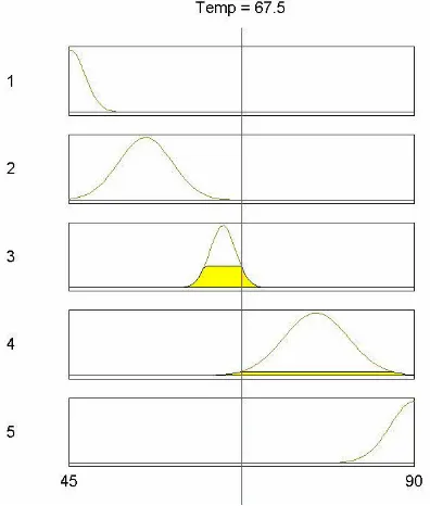
Fig. 3 shows the input variable (temperature) membership functions. We have chosen them to be of Gaussian bell shape.
Fig. 4 shows the output variable (fan speed) membership functions. We have chosen them to be of triangular shape.
Once the training is completed, the system becomes ready for testing. The testing is represented by feeding the controller with temperature values and monitoring the resulting decision generated by it. One of the testing examples is shown in figs. 5a and 5b. If we select the input temperature to be 67.5 Fo, the resulting fan speed would be 55.9 rpm.
The set of rules that links input membership functions to the output ones is:
1. if (Temp is Cold) then (Speed is Stop) 2. If (Temp is Cool) then (Speed is Slow) 3. If (Temp is Optimal) then (Speed is Medium) 4. If (Temp is Hot) then (Speed is Fast)
5. If (Temp is Very Hot) then (Speed is Blast)
The temperature 67.5 Fo is common to both ‘optimal’ and ‘hot’ input membership functions. However it is more towards the ‘optimal’ one (note the shaded areas in fig. 5a). The corresponding output membership functions are fired according to the five rules given earlier. Accordingly, they are ‘medium’ and ‘fast’. The final crisp value for the speed selection is done by a process called defuzzification [7]. In this process, the centroid [8][9] of the output membership shaded areas is calculated. In our case this results in 55.9 rpm.
[image:3.612.317.522.89.406.2]Fig. 6 shows the overall surface relationship between the temperature applied and the resulting fan speed.
Fig. 3. Temperature membership functions.
[image:3.612.72.297.293.405.2]Fig. 4. Fan speed membership functions.
Fig. 5a. Input temperature sensed is 67.5 Fo
Fig. 5b. Resulting fan speed is 55.9 rpm.
[image:3.612.84.282.498.731.2]Fig. 6 represents a planar relationship between the temperature and the fan corresponding speed. If we add another input (like room humidity) and make it part of the speed decision, the said relationship becomes three dimensional surface.
V. EPASFUZZY CONTROLLER
In this section, we train a fuzzy controller to substitute the original H∞ controller. The design details of the H∞ controller are far beyond the scope of this paper. However, we refer to the controller signals as needed. The original controller receives three signals: Tc, Theta_c, and Theta_m_dot and produces one control signal U [3]. Figs. 7 and 8 show the said input and output signals
0 0.5 1 1.5 2
-4000 -2000 0 2000 4000
Time (s)
O
ri
g
in
a
l
C
o
n
tr
o
ll
e
r
In
p
u
t
S
ig
n
a
ls
Tc Theta c Theta m dot
0 0.5 1 1.5 2
-10 -5 0 5 10
Time (s)
O
ri
g
in
a
l
C
o
n
tr
o
ll
e
r
O
u
tp
u
t
S
ig
n
a
l U
One of the important training issues for fuzzy controllers is the number of membership functions and the shape of the said functions. In this paper we use three fuzzy controllers, one for each input. The over all performance will be the average of the three controllers. Further tuning is possible to make the contribution of one controller exceeds the others, i.e. one the controllers will the dominant over the other two ones.
The fuzzy controllers training parameters are as follows:
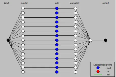
Number of nodes: 64
Number of linear parameters: 30 Number of nonlinear parameters: 45 Total number of parameters: 75 Number of training data pairs: 41055 Number of checking data pairs: 0 Number of fuzzy rules: 15
We choose the same structure for all of the three fuzzy controllers. The said structure is shown in fig. 9.
Figs 10a, 10b, and 10c show the membership function distributions of the fuzzy controller inputs Tc, Theta_c, and Theta_m_dot. The fuzzy controller overall output signal would be the average of the three outputs.
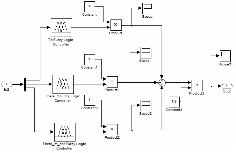
Fig. 11 shows the three fuzzy controllers and the way they are connected to produce the overall control signal U. We can
see that the controllers have the same effect on the overall control signal. The system performance could be further improved by changing the controller weights (they are currently set to 1). In other words we can make the contribution of one or two of the controllers exceed that of the others by changing their weights. However, it is an experimental method and it does not have analytical bases as of yet.
[image:4.612.313.542.149.300.2][image:4.612.314.541.490.589.2]
Fig. 7. H∞ controller input signals.
Fig. 8. H∞ controller output signal.
Fig. 9. Fuzzy controllers structure.
Fig. 10a. Tc signal membership function distribution.
[image:4.612.313.539.630.730.2]Fig. 10b. Theta_c signal membership function distribution.
VI. FUZZY CONTROLLER SIMULATION RESULTS
Once the fuzzy controller is trained, it becomes ready to replace the original H∞ system. The overall system is shown in fig. 12.
Fig. 12 shows the overall control system based on the fuzzy controller. The original H∞ controller is completely removed and replaced with the fuzzy one.
Fri ctio n co mpen sator
den(s) 1
T dest
T d esti [T,Td]
T d
th mdo t theta
T cest Tc esti T c
T adesi red
T a 0.02s+1
0.001 s+1 Predi ctor
x' = Ax+Bu y = Cx+Du
PLANT 40 Gai n1 40 Gai n theta u Tdest Tcest Esti mators Tc Theta_c Theta_m_dot Ta desired Td U
Equi li bri um
In2 Out2
EPAS Fuzzy Co ntroll er Demux
den(s) 1
We need to see now, how the new system would behave when exposed to the road conditions and driver’s steering torque. The driver’s steering torque is applied via an external driver torque signal generator (Td). Then, we measure the assist torque (both desired and actual). The difference between the two represents the error signal that we try to minimize. Figs 13-16 show the applied torque and the assist torque in both of the H∞ controller and its corresponding fuzzy one.
0.2 0.4 0.6 0.8 1 1.2 1.4 1.6 1.8 2 -40 -20 0 20 40 Time (s) T a a n d T a d e s ir e d (H i n fi n it y C o n tr o ll e r) Ta Tadesired
0.2 0.4 0.6 0.8 1 1.2 1.4 1.6 1.8 2 -10 -5 0 5 T a T a d e s ir e d (H i n fi n it y C o n tr o ll e r) Time (s)
0.2 0.4 0.6 0.8 1 1.2 1.4 1.6 1.8 2 -40 -20 0 20 40 Time (s) T a a n d T a d e s ir e d (F u z z y C o n tr o ll e r) Ta Tadesired
0.2 0.4 0.6 0.8 1 1.2 1.4 1.6 1.8 2 -10 -5 0 5 10 T a - T a d e s ir e d (F u z z y C o n tr o ll e r) Time (s)
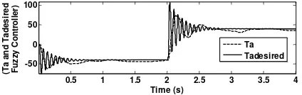
It would be also useful to test the system against harsh driving circumstances. Driving a car is not always a smooth process. The driver sometimes needs to make sudden decisions to avoid certain obstacles that may appear along his/her way. Sudden steering is an example of these harsh circumstances.
Figs 17 and 18 show the performance of the H∞ system. One can notice the fluctuation in (Ta) value once the step torque is applied. This fluctuation damps with time shortly and the system reaches its steady state.
0.5 1 1.5 2 2.5 3 3.5 4
-50 0 50 100 Time (s) T a a n d T a d e s ir e d (H I n fi n it y C o n tr o ll e r) Ta Tadesired
0.5 1 1.5 2 2.5 3 3.5 4
-100 -50 0 50 T a T a d e s ir e d (H I n fi n it y C o n tr o ll e r) Time (s)
[image:5.612.71.304.111.262.2]Figs 19 and 20 show the performance of the fuzzy control system. We can notice that both of the systems are almost
Fig. 11. EPAS System fuzzy controller.
[image:5.612.75.292.355.483.2]Fig. 12. Fuzzy controller based EPAS system.
Fig. 13. H∞ Ta and Ta desired signals.
Fig. 14. H∞ Ta-Ta desired signals.
Fig. 16. Fuzzy controller Ta-Ta desired signal. Fig. 15. Fuzzy controller Ta and Ta desired signals.
Fig. 17. H∞ Ta and Ta desired signals in response to driver’s step
Steering.
identical and both reach the same level of stability (steady state error) at the same time.
0.5 1 1.5 2 2.5 3 3.5 4
-50 0 50 100
Time (s)
(T
a
a
n
d
T
a
d
e
s
ir
e
d
F
u
z
z
y
C
o
n
tr
o
ll
e
r)
Ta Tadesired
0.5 1 1.5 2 2.5 3 3.5 4
-100 -50 0 50
T
a
T
a
d
e
s
ir
e
d
(F
u
z
z
y
C
o
n
tr
o
ll
e
r)
Time (s)
VII. CONCLUSIONS AND FUTURE WORK
The major conclusion we come to in this paper, is the ability of fuzzy systems to play the role of EPAS controllers. We have noticed that the performance of the fuzzy controller is almost identical with that of the original H∞ one. The choice of appropriate fuzzy parameters like the number and shape of membership functions plays an important role in realizing this identity. With small number of functions, the error rate will increase but the system complexity will be smaller and vice versa. It is well known that the higher the complexity of the system, the slower the overall response to be. Our future work will be focusing on finding methods and/or algorithms that help in deciding the optimal number and perhaps the optimal shape of the membership functions. We need to reach certain level of fuzzy system complexity so that the error would be the best, and the response would be the fastest.
REFERENCES
[1] R. Chabaan, “Torque Estimation in Electrical Power Steering Systems,”
IEEE Vehicle Power and Propulsion Conference, Dearborn, MI, Sep. 2009.
[2] R. Chabaan, “Optimal Control and Gain Scheduling of Electrical Power
Steering Systems,” IEEE Vehicle Power and Propulsion Conference,
Dearborn, MI, Sep. 2009.
[3] R. Kenaya and R. Chabaan, “Neural Controllers for Electrical Power
Steering Systems,” IEEE International Conference on
Electro/Information Technology, Normal, IL, May, 20-22, 2010.
[4] R. Kenaya and K. Cheok, “Euclidean ART Neural Networks,” World
Congress on Engineering and Computer Science Proceedings, pp.
963-968, October 2008,San Francisco.
[5] J. –S. R. Jang, C. T. Sun, and E. Mizutani, Neuro Fuzzy and Soft
Computing. Prentice Hall, 1997.
[6] B. Kosko, Neural Networks and Fuzzy Systems, Prentice Hall, 1992.
[7] S. Rivera, J. Mc Leod, “RMS Defuzzification Algorithms Applied To
FMEA,” 8th. World Congress on Computational Mechanics (WCCM8),
June 30 – July 5, 2008, Venice, Italy.
[8] S. Opricovic and G. Tzeng, “Defuzzification within a Multicriteria
Decision Model,” International Journal of Uncertainty, Fuzziness and
Knowledge-Based Systems, vol. 11, No. 5 (2003) 635-652.
[9] A. Lorestani, M. Omid, S. Bagheri Shooraki, A.M. Borghei and A.
Tabatabaeefar, “Design and Evaluation of a Fuzzy Logic Based Decision
Support System for Grading of Golden Delicious Apples,” International
Journal Of Agriculture & Biology, 1560–8530/2006/08–4–440–444.
[image:6.612.73.285.85.152.2]
Fig. 19. Fuzzy controller Ta and Ta desired signals in response to driver’s step Steering.