Hearing-Aid Android Application using Machine
Learning
Pratik Giri1, Viraj Rajderkar2, Mandar Sadye3, Siddhesh Sharma4, Rajesh Patil5
1, 2, 3, 4Student, Department of Electrical Engineering, Veermata Jijabai Techological Institute
5Professor, Department of Electrical, Veermata Jijabai Technological Institute
Abstract: This paper presents the configuration, digital signal processing and machine learning details of an Android-based hearing aid application connected to standard earphones, whereby the smartphone performs full sound processing and inference of neural network rather than solely providing a means of setting adjustment by streaming to conventional digital hearing aids. Keywords: Hearing Aid, Machine Learning, Android Application, Speech Processing
I. INTRODUCTION
There has been a rapid development in the technology of hearing aids since DSP was introduced in 1996 [1–6]. However, a significant number of hearing aid wearers continue to be dissatisfied in many key areas such as sound naturalism, clarity, soft sound, inaudibility etc [1–6] . Some of the limitations are because of the fact that every amplifier has response limitations (e.g., in relation to frequency or bandwidth, phase and slew-rate), and such limitations are to be especially expected within the confines of miniaturization of the hearing aid. One of the major factors in the degradation of the quality and intelligibility of speech signals is the presence of background noise, which the conventional hearing aids are not very efficient at removing. This problem of separating the human speech from background noise is termed as speech enhancement problem.
More recently, application of data-driven methods to the speech enhancement problem has attracted considerable interest. The expectation is that after providing with sufficient training data, a suitable model can learn the underlying complex statistical relationships between the speech and corrupting noise signals. Some of the hearing aid manufacturers are beginning to implement data driven approaches in their hearing aid equipments, but, the cost of these sophisticated hearing aids is very high. This causes the average customer to stick to conventional DSP hearing aids with poor speech enhancement abilities. Smartphones on the other hand are widely used by a large number of people, and an application can be installed without any additional cost. Therefore, this paper discusses the implementation of hearing aid using machine learning approaches on an android smartphone.
II. ARCHITECTURE OF BACKEND CODE
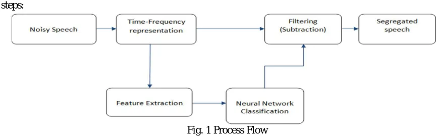
[image:1.612.81.519.508.643.2]In this section we discuss the algorithms used in the backend of the android application. The process can be divided into the following steps:
Fig. 1 Process Flow
A. Sampling
Android devices using the provided APIs. Input latency is between 100ms and 250ms for a typical android phone. We also need to ensure that the system will work with most phones. Therefore, the recording rate was set at 900ms since the input latency cannot be reduced in any given device. A sampling rate of 44100 Hz, mono format and 16 bit encoding is supported on most of the devices according to the android platform specifications. The requirements for human hearing application can be satisfied with this format of audio.
B. Time-Frequency Transformation
This step provides us with the frequency information present in a particular interval of time which is further used as input to the neural network block after necessary feature extraction. We have used wavelet transform for this particular application. Since the wavelet transform is known to be very convenient for application in speech processing.
C. Feature Extraction
The biggest challenge in signal processing is whether all of the information necessary to distinguish words can be preserved during the feature extraction stage or not. If important information is missing after this stage, the performance of the next classification stage is inherently damaged and can never measure up to human capability. Feature extraction is nothing but a step to reduce the dimensionality of the input data, which inevitably leads to some information loss. The mel-cepstrum feature, which is based on human auditory perception, has been used extensively for speech processing. Typically, the mel-cepstrum is obtained using critical band filters. Hence, the parameters of the critical filters, like center frequencies and bandwidths, can be optimized to reduce the rate of error in speech recognition. The optimization of these parameters can be done by finding the minimum of a function whose inputs are the parameters of the filters and whose output is the error rate.
D. Neural Network Block
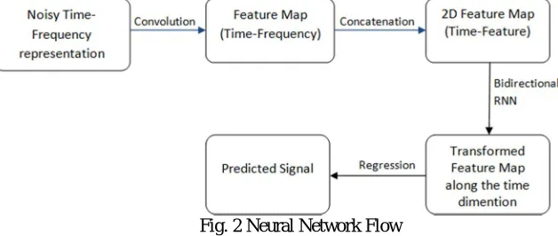
[image:2.612.137.451.406.539.2]In this section we introduce the proposed model, in detail and discuss its design principles as well as its bias toward solving the enhancement problem. At a high level, we view the enhancement problem as a multivariate regression problem, where the nonlinear regression function is parameterized by the network in Fig. 2. Alternatively, the whole network can be interpreted as a complex filter for noise reduction in the frequency domain.
Fig. 2 Neural Network Flow
1) Convolutional Component: The denoising function g can be chosen as multilayer perceptrons, which has been extensively explored in the past few years. [7–10] The fully connected network structure of MLPs are universal function approximators. But inspite of that they usually cannot exploit the rich patterns existing in spectrograms. This key observation motivates us to apply convolutional neural networks to efficiently and cheaply extract local patterns from the input spectrogram. The convolution kernels’ application is particularly well suited for speech enhancement in the frequency domain because each kernel can be understood as a nonlinear filter that detects a specific kind of local patterns existed in the noisy spectrograms, and the width of the kernel has a natural interpretation as the length of the context window. On the computational side, since convolution layer can also be understood as a special case of fully- connected layer with shared and sparse connection weights, the introduction of convolutions can thus greatly reduce the computation needed by an MLP with the same expressive power.
from the previous convolutional feature map. We use deep bidirectional long short-term memory (LSTM) as our recurrent component due to its ability to model long-term interactions. At each time step t, given input Ht(x), each unidirectional LSTM cell computes a hidden representation. To build deep bidirectional LSTMs, we can stack additional LSTM layers on top of each other.
3) Fully-connected Component and Optimization: Let H~(x) be the output of the bidirectional LSTM layer. To obtain the estimated clean spectrogram, we apply a linear regression with truncation (removal of some part) to H~(x) such that we ensure the prediction lies in the non negative orthant. As discussed earlier, the last step is to define the mean-squared error between the predicted spectrogram and the clean one, and optimize all the model parameters simultaneously.
E. Filtering (Subtraction)
Finally, we obtain the spectrogram of the noise at the output of the neural network block. To obtain the spectrogram of the clean speech, we need to subtract the noise spectrogram from the original spectrogram. This output is the final clean speech spectrogram.
III. ANDROID IMPLEMENTATION
In the app, we used NDK instead of SDK. It allows programing in C/C++ for Android devices. As the code is written in C or C++ it is generally faster than its JAVA counterpart. It enables performance and latency can be controlled in the range of milliseconds. As this application had many complex calculations to be performed with latency as low as possible it was found that it is more suitable to use NDK for the most part of the code.
A. Latency
There are two major reasons for latency: Latency induced by the device hardware and operating system and latency induced by the application. We are going to focus on the later part in this section. The former part cannot be changed by the application developer for a given device.
The most basic solution is to remove all the unnecessary software layers. To implement this solution, Android NDK was used which removes the JVM layer and provides significant improvement in performance. To access audio with minimum possible latency, Google’s Oboe library was used for audio input and output. This library uses kernel level threads to access the microphones and other audio jack. Oboe uses different API’s written in native C/C++ language.
Audio latency induced by the app is the sum of processing delay of the sequential operations performed in the backend stage. Processing delay includes operations like memory access. Therefore, evaluation of every operation must be done and unnecessary operations must be removed. The remaining operations must be optimally designed. For example, unnecessary copies of objects should be avoided by use of pointers.
B. Format for Saving Audio
The WAV format is used for saving the audio in our project. This was chosen because, most supported formats either employ perceptual coding or have low sampling rate. Additional work is required to save the audio in any other common format, whereas WAV-format is lossless non-packed format. It stores raw audio
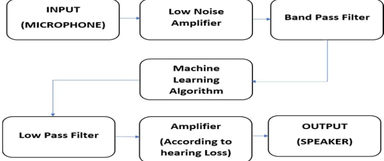
[image:3.612.115.499.557.718.2]In the final version of the app, microphone buffer data is directly used and no storing is necessary. But, saving audio data is invaluable for debugging and demonstration purposes.
IV. RESULTS A. Result of Neural Network
1) Dataset: The used dataset was generated from two sources: speech data was supplied by the Voice Bank corpus while environmental sounds were provided by the Diverse Environments Multichannel Acoustic Noise Database (DEMAND). The subset of the Voice Bank corpus we used features 30 native English speakers from different parts of the world reading out ≈
400 sentences – 28 speakers are used for training and 2 for testing. Recordings are of studio quality sampled at 48 kHz – and subsampled to 16 kHz for this study. The subset of DEMAND that we used provides recordings in 13 different environmental conditions such as in a park, in a bus or in a cafe – 8 background-noises are mixed with speech during training and 5 background-noises are used during testing. DEMAND was produced with a 16-channel array sampled at 48 kHz, however for the purposes of this work all channels were merged and subsampled to 16 kHz. During training, two artificial noise classes were added – in total 10 different noise classes are available during training. Training samples are synthetically mixed at one of the following four signal-to-noise ratios (SNRs): 0, 5, 10 and 15dB with one of the 10 noise types. This results in 11,572 training samples from 28 speakers under 40 different noise conditions. Test samples are also synthetically mixed at one of the following four different SNRs: 2.5, 7.5 and 17.5dB with one of the 5 test-noise types – resulting in 20 noise conditions for 2 speakers. As a result, the test set features 824 samples from unseen speakers and noise conditions. For both sets, the samples are on average 3 seconds long with a standard deviation of 1 second. No pre-processing to the audio is used.
2) Quantitative Analysis: Signal-to-noise ratio (SNR) is a measure that compares the level of a desired signal to the level of background noise. SNR is defined as the ratio of signal power to the noise power, often expressed in decibels. A ratio higher than 1:1 (greater than 0 dB) indicates more signal than noise.
SNRdB=10
The ideal SNR of the signal was calculated as follows
a)The clean speech and the background noise powers were calculated separately.
b)Their ratio was calculated as SNRoriginal.This is the ideal SNR since it is calculated using clean speech separately.
c)The noisy speech (Clean speech + background noise) was passed through the model and output speech was obtained.
d)The power of this output signal was calculated and SNR was calculated.
3) Interpretation of the Results
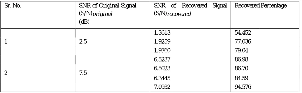
a) Since the original SNR is the maximum possible SNR that can be recovered, therefore the obtained SNR is compared to this value and the percentage of the signal that was recovered was calculated.
b) The closer the obtained SNR gets to the ideal case, the better the result.
[image:4.612.49.567.528.689.2]c) It was observed that the signal recovery percentage increases with increase in original SNR. This is because the neural network is able to classify noise with better accuracy under low noise conditions.
TABLE I
SNR Original Vs Recovered Sr. No. SNR of Original Signal
(S/N)original
(dB)
SNR of Recovered Signal (S/N)recovered
Recovered Percentage
1.3613 54.452
1 2.5 1.9259 77.036
1.9760 79.04
6.5237 86.98
2 7.5 6.5023
6.3445
86.70
84.59
7.0932 94.576
Table I continued
Sr. No. SNR of Original Signal (S/N)original
(dB)
SNR of Recovered Signal (S/N)recovered
Recovered Percentage
11.7434 93.9472
3 12.5 11.0020 88.016
12.1997 97.5976
16.7358 95.633
4 17.5 16.4676 94.100
17.0177 97.244
B. Android Application
1) Explanation of the Interface: First connect the headphones to the audio jack of the device and open the app. Select the appropriate values for all the fields according to the following:
a) Recording Device: This field can be used to select the microphone which will sample the input audio signal
b) Playback Device: This field can be used to select the output device which will play the clean audio. Headphones are selected by default
c) Select Filter: This can be used to turn off the machine learning algorithm. This can be useful to find the difference in the quality of speech enhancement.
d) Amplitude: A slider is provided to vary the amplitude of the output audio
e) Start Button: This button is used to start or stop the backend core of the app
V. CONCLUSION
This paper proposes a Hearing Aid Android Application which uses signal processing and machine learning approaches to isolate human speech from noisy input audio in bounded latency. Most importantly, the solution proposed in this thesis can be used on existing smartphone devices without requiring any modifications in the hardware. Further, we can expect a better performance in the future as the audio quality supported by mobile devices continues to increase.
These type of applications have enormous potential in the future given the realms of machine learning and artificial intel- ligence are expanding rapidly in every domain. Efficient Data processing techniques are being developed and this system can be further developed by integrating these techniques (such as bit-precision scaling), thus improving computation speed, thereby reducing the time latency required in inference stage of the neural network.
REFERENCES
[1] “Edwards B. The future of hearing aid technology,” Trends Amplif, vol. 11, pp. 31–45.
[2] “Ingrao B. Getting it right the first time, best practices in hearing aid fitting,” Hear Loss Magazine, no. 14-8, 2012, Jan/Feb.
[3] “McPherson B. Innovative technology in hearing instruments: Matching needs in the developing world,” Trends Amplif, vol. 15:209-14, 2011. [4] J. Agnew, “Acoustic feedback and other audible artefacts in hearing aids,” pp. 45–82, 1996.
[5] S. Kochkin, “MarkeTrak V: “Why my hearing aids are in the drawer”: the consumer’s perspective,” Hear J, pp. 34–41, 2000. [6] Kochkin, “MarkeTrak VIII: Consumer satisfaction with hearing aids is slowly increasing,” Hear J, vol. 63, pp. 19–32, 2005.
[7] X. Lu, Y. Tsao, S. Matsuda, and C. Hori, “Speech enhancement based on deep denoising autoencoder” , pp. 436–440, 2013, in Interspeech.
[8] Y. Xu, J. Du, L.-R. Dai, and C.-H. Lee, “Chin-Hui Lee, “An experimental study on speech enhancement based on deep neural networks,”,” pp. 65–68, 2014. [9] Yong, J. Du, L.-R. Dai, and C.-H. Lee, “A regression approach to speech enhancement based on deep neural networks,”, pp. 7–19, 2015.