Improved Estimation of Entropy for Evaluation of Word Sense Induction

Evaluation of Word Sense Induction

Linlin Li

Microsoft Development Center Norway

Ivan Titov

University of Amsterdam

Caroline Sporleder

Information-theoretic measures are among the most standard techniques for evaluation of clustering methods including word sense induction (WSI) systems. Such measures rely on sample-based estimates of the entropy. However, the standard maximum likelihood estimates of the entropy are heavily biased with the bias dependent on, among other things, the number of clusters and the sample size. This makes the measures unreliable and unfair when the number of clusters produced by different systems vary and the sample size is not exceedingly large. This corresponds exactly to the setting of WSI evaluation where a ground-truth cluster sense number arguably does not exist and the standard evaluation scenarios use a small number of instances of each word to compute the score. We describe more accurate entropy estimators and analyze their performance both in simulations and on evaluation of WSI systems.

1. Introduction

The task of word sense induction (WSI) has grown in popularity recently. WSI has the advantage of not assuming a predefined inventory of senses. Rather, senses are induced in an unsupervised fashion on the basis of corpus evidence (Sch ¨utze 1998; Purandare and Pedersen 2004). WSI systems can therefore better adapt to different target domains that may require sense inventories of different granularities. However, the fact that WSI systems do not rely on fixed inventories also makes it notoriously difficult to evaluate and compare their performance. WSI evaluation is a type of cluster evaluation problem. Although cluster evaluation has received much attention (see, e.g., Dom 2001; Strehl and Gosh 2002; Meila 2007), it is still not a solved problem. Finding a good way to score partially incorrect clusters is particularly difficult. Several solutions have been

∗Microsoft Development Center Norway. E-mail:[email protected].

∗∗Institute for Logic, Language and Computation. E-mail:[email protected].

†Computational Linguistics and Digital Humanities, Trier University, 54286 Trier, Germany.

E-mail:[email protected].

Submission received: 14 March 2013; revised version received: 13 September 2013; accepted for publication: 20 November 2013

proposed but information theoretic measures have been among the most successful and widely used techniques. One example is the normalized mutual information, also known as V-measure (Strehl and Gosh 2002; Rosenberg and Hirschberg 2007), which has, for example, been adopted in the SemEval 2010 WSI task (Manandhar et al. 2010).

All information theoretic measures of cluster quality essentially rely on sample-based estimates of entropy. For instance, the mutual information I(c, k) between a gold standard class c and an output cluster k can be written H(c)+H(k)−H(k, c), where H(c) and H(k) are the marginal entropies of c and k, respectively, and H(k, c) is their joint entropy. The most standard estimator is the maximum-likelihood (ML) estimator, which substitutes the probability of each event (cluster, classes, or cluster-class pair occurrence) with its normalized empirical frequency.

Entropy estimators, even though consistent, are biased. This means that the expected estimate of the entropy on a finite sample set is different from the true value. It is also different from an expected estimate on a larger test set generated from the same distribution, as the bias depends on the size of the sample. This discrepancy negatively affects entropy-based evaluation measures, such as the V-measure. This is different from supervised classification evaluation, where the classification accuracy on a finite test set is expected to be equal to the error rate (for the independent and identically distributed, i.i.d.) case, though it can be different due to variance (due to choice of the test set). As long as the number of samples is large with respect to the number of classes and clusters, the estimate is sufficiently close to the true entropy. Otherwise, the quality of entropy estimators matters and the bias of the estimator can be large. This problem is especially prominent for the ML estimator (Miller 1955).

In WSI, we are faced with exactly those conditions that negatively affect the entropy estimators. In a typical setting, the number of examples per word is small—for example, less than 100 on average for the SemEval 2010 WSI task. The number of clusters, on the other hand, can be fairly high, with some systems outputting more than 10 sense clusters per word on average. Because the bias of an entropy estimator is dependent on, among other things, the number of clusters, the ranking of different WSI systems is partly affected by the number of clusters they produce. Even worse, the ranking is also affected by the size of the test set. The problem is exacerbated when computing the joint entropy between clusters and classes, H(k, c), because this requires estimating the joint probability of cluster-class pairs for which the statistics are even more sparse.

The bias problem of entropy estimators has long been known in the information theory community and many studies have addressed this issue (e.g., Miller 1955; Batu et al. 2002; Grasberger and Sch ¨urmann 1996). In this article, we compare different estimators and their influence on the computed evaluation scores. We run simulations using a Zipfian distribution where we know the true entropy. We also compare different estimators against the SemEval 2010 WSI benchmark. Our results strongly suggest that there are estimators, namely, the best-upper-bound (BUB) estimator (Paninski 2003) and jackknifed (Tukey 1958; Quenouille 1956) estimators, which are clearly preferable to the commonly used ML estimators.

2. Clustering Evaluation

2.1 Information-Theoretic Measures

and the gold-standard classes. A natural approach would be to consider arbitrary statistical dependencies between the cluster assignment k and the class assignment c. The standard measure of statistical dependence of two random variables is the Shannon mutual information I(k, c) (MI). MI is 0 if two variables are independent, and it is equal to the entropy of a variable if another variable is deterministically dependent on it. Clearly, such measure would favor clusterings with higher entropy, and, consequently, normalized versions of MI are normally used to evaluate clusterings. One instance of normalized MI actively used in the context of WSI evaluation is the V-measure, or symmetric uncertainty (Witte and Frank 2005; Rosenberg and Hirschberg 2007):

V(k, c)= 2I(k, c) H(k)+H(c) =

2(H(k)+H(c)−H(k, c)) H(k)+H(c)

though other forms of MI normalization have also been explored (Strehl and Gosh 2002). Because the true marginal and the joint entropies are not known, the standard maximum likelihood estimators (also called plug-in estimators of entropy) are normally used instead. The ML estimates ˆH have the analytical form of an entropy with the normalized empirical frequency substituted instead of the unknown true membership probabilities, for example:

ˆ H(c)=

m

i=1 −ni

Nlog ni

N (1)

where niis the number of times cluster i appears in the set, m is the number of clusters,

and N is the size of the set (i.e., the sample size).

The ML estimators of entropy are consistent but heavily negatively biased (see Section 3 for details). In other words, the expectation of ˆH is lower than the true entropy, and this discrepancy increases with the number of clusters m and decreases with the sample size N. When m is comparable to N, the ML estimator is known to be very inaccurate (Paninski 2004).

Note that for V-measure estimation the main source of the estimation error is the joint entropy H(k, c),1as the number of possible pairs (c, k) for most systems would be large whereas the total number of occurrences will remain the same as for the estimation of H(c) and H(k). Therefore, the absolute value of the bias for ˆH(c, k) will exceed the aggregate bias of the estimators of marginal entropy, ˆH(c) and ˆH(k). As a result, the V-measure will be positively biased, and this bias would be especially high for systems predicting a large number of clusters.

This phenomenon has been previously noticed (Manandhar et al. 2010) but no satis-factory explanation has been given. The shortcomings of the ML estimator are especially easy to see on the example of a baseline system that assigns every instance in the testing set to an individual cluster. This baseline, when averaged over the 100 target words, out-performs all the participants’ systems of the SemEval-2010 task on the standard testing set (Manandhar and Klapaftis 2009). Though we cannot compute the true bias for any real system, the computation is trivial for this baseline. The true V-measure is equal to 0,

as the baseline can be regarded as a limiting case of a stochastic system that picks up one of the m clusters under the uniform distribution with m→ ∞; the mutual information between any class labels and clustering produced by such model equals 0 for every m. However, the ML estimate for the V-measure is ˆV(k, c)=2 ˆH(c)/(log N+H(c)). For theˆ testing set of SemEval 2010, this estimate, averaged over all the words, yields 31.7%, which by far exceeds the best result of any system (16.2%). On an infinite (or sufficiently large) set, however, its performance would change to the worst. This is a problem not only for the baseline but for any system which outputs a large number of classes: The error measures computed on the small test set are far from their expectations on the new data. We will see in our quantitative analyses (Section 5) that using more accurate estimators will have the most significant effect on both the V-measure and on the ranks of systems which output richer clustering, agreeing with this argument.

Though in this analysis we focused on the V-measure, other information theoretic measures have also been proposed. Examples of such measures include the variation of information measure (Meila 2007) VI(c, k)=H(c|k)+H(k|c) and Q0 measure (Dom 2001) H(c|k). This argument applies to these evaluation measures as well, and they can all be potentially improved by using more accurate estimators.

2.2 Alternative Measures

Not only information-theoretic measures have been proposed for clustering evaluation. An alternative evaluation strategy is to attempt to find the best possible mapping between the predicted clusters and the gold-standard classes and then apply standard measures like precision, recall, and F-score. However, if the best mapping is selected on the test set the result can be overoptimistic, especially for rich clusterings. Consequently, such methods constrain the set of permissible mappings to a restricted family. For exam-ple, for the F-score, one considers only mappings from each class to a single predicted cluster (Zhao and Karypis 2005; Agirre and Soroa 2007). This restriction is generally too strong for many clustering problems (Meila 2007; Rosenberg and Hirschberg 2007), and especially inappropriate for the WSI evaluation setting, as it penalizes sense induction systems that induce more fine-grained senses than the ones present in the gold-standard sense set.

The Paired F-score (Manandhar et al. 2010) is somewhat less restrictive than the F-score measures in that it defines precision and recall in terms of pairs of instances (i.e., effectively evaluating systems based on the proportion of correct links). However, the Paired F-score has the undesirable property that it ranks those systems highest which put all instances in one cluster, thereby obtaining perfect recall.

As an alternative, the supervised evaluation measure has been proposed (Agirre et al. 2006). This approach in addition to the testing set uses an auxiliary mapping set. First the mapping is induced on the mapping set, then the quality of the mapping is evaluated on the testing set. One problem with this evaluation scenario is that the size of the mapping set has an effect on the results and there is no obvious criterion for selecting the right size of the mapping set. For the WSI task, the importance of the set size was empirically confirmed when the evaluation set was split in proportions 80:20 (80% for the mapping sets, and 20% for testing) instead of the original 60:40 split: The scores of all top 10 systems improved and the ranking changed as well (Manandhar et al. 2010) (see also Table 1 later in this article).

For a more general assessment of measures for clustering evaluation see Amigo et al. (2009) and Klapaftis and Manandhar (2013).

3. Entropy Estimation

Given the influence that information theory has had on many fields, including signal processing, neurophysiology, and psychology, to name a few, it is not surprising that the topic of entropy estimation has received considerable attention over the last 50 years.2 However, much of the work has focused on settings where the number of classes is significantly lower than the size of the sample. More recently a set-up where the sample size N is comparable to the number of classes m has started to receive attention (Paninski 2003, 2004).

In this section, we start by discussing the intuition for why the ML estimator is heavily biased in this setting. Though unbiased estimators of entropy do not exist,3 various techniques have been proposed to reduce the bias while controlling the vari-ance (Grasberger and Sch ¨urmann 1996; Batu et al. 2002). We will discuss widely used bias-corrected estimators, the ML estimator with Miller-Madow bias correction (Miller 1955) and the jackknifed estimator (Strong et al. 1998). Then we turn to the more recent technique proposed specifically for the N∼m setting, the best-upper-bound (BUB) estimator (Paninski 2003). We will conclude this section by explaining how these estimators can be computed using stochastic (weighted) output of WSI systems.

3.1 Standard Estimators of Entropy

As we discussed earlier, the ML estimator (1) is negatively biased. For a fixed distri-bution p, a little algebra can be used to show that the bias of the maximum likelihood estimator can be written as

H−Ep( ˆH)=Ep(D( ˆpp))

where Ep denotes an expectation under p, D is the Kullback-Leibler (KL) divergence,

and ˆp is the empirical distribution in the sample of N elements drawn i.i.d. from p. Because the KL-divergence is always non-negative, it follows that the bias is always non-positive. It also follows that the expected divergence is larger if the size of the sample is small. In fact, this expression can be used to obtain the asymptotic bias rate (N→ ∞) (Miller 1955). The bias rate derived in this way would suggest a form of correction to the ML estimator, called Miller-Madow bias correction ˆHMM=Hˆ +mˆ−N1,

where ˆm is an estimate of m, as the true size of support m may not be known. In our experiments, we use a basic estimator ˆm which is just the number of different clusters (classes or cluster-class pairs depending on the considered entropy) appearing in the sample. We will call the estimator ˆHMMthe Miller-Madow (MM) estimator. As the MM

estimator is motivated by the asymptotic behavior of the bias, it is not very appropriate for N∼m.

2 For a relatively recent overview of progress in entropy estimation research see, for example, the proceedings of the NIPS 2003 workshop on entropy estimation.

The bias of the ML estimator decreases with the size of the sample. Intuitively, an estimate of the discrepancy in estimates produced from samples of different sizes can be used to correct the ML estimator: If an estimate based on N−1 samples significantly exceeds the estimate from N samples, then the bias of the estimator is still large. Roughly, this intuition is encoded in the jackknifed (JK) estimator (Strong et al. 1998):

ˆ

HJK=N ˆH−N_N−1 N

j=1 ˆ H−j

where ˆH−jis the ML estimator based on the original sample excluding the example j.

3.2 BUB Estimator

We can observe that all the previous estimators can be expressed in the form of a linear function of the ordered histogram statistics

ˆ H(aaa)=

N

j=0

aj,Nhj (2)

where hjis the number of classes which appear j times in the sample:

hj= m

i=1

[[ni=j]] (3)

where [[ ]] denotes the indicator function. The coefficients aj,Nfor the ML, MM, and JK

estimators are equal to:

aML,j,N =− j Nlog

j N

aMM,j,N =−_Nj log_Nj + 1−_Nj

N

aJK,j,N =NaML,j,N−N_N−1((N−j)aML,j,N−1+jaML,j−1,N−1)

This observation suggests that it makes sense to study an estimator of the general form ˆH(aaa) as defined in Equation (2). Upper bounds on the bias and variance of such estimators4 _{have been stated in Paninski (2003). These bounds imply an upper bound} on the standard measure of estimator performance, mean squared error (MSE, the sum of the variance and squared bias). The worst-case estimator is then obtained by selecting aaa to minimize the upper bound on MSE, and, therefore, it is called the best-upper-bound estimator. This optimization problem5 _{corresponds to a regularized}

4 We argued that variance is not particularly important for the ML estimator with N∼m. However,

for an arbitrary estimator of the form of Equation (2) this may not be true, as the coefficients aj,N may be oscillating, resulting in an estimator with a large variance (Antos and Kontoyiannis 2001).

5 More formally, its modification where the L2norm is optimized instead of the original L∞

least-squares problem and can be solved analytically (see Appendix A and Paninski [2003] for technical details).

This technique is fairly general, and can potentially be used to minimize the bound for a particular type of distribution. This direction can be promising, as the types of distributions observed in WSI are normally fairly skewed (arguably Zipfian) and tighter bounds on MSE may be possible. In this work, we use the universal worst-case bounds advocated in Paninski (2003).

3.3 Estimation with Stochastic Predictions

As many WSI systems maintain a distribution over predicted clusters, in SemEval 2010 the participants were encouraged to provide a weighted prediction (i.e., a distribution over potential clusters for each example) instead of predicting just a single most-likely cluster.

We interpret the weighted output of a system on an example l as a categorical trial with the probabilities of outcomes ˜p_i(l)provided by the model where i is an index of the cluster. Therefore a stochastic output of a system on the test set represents a distribution over samples generated from these trials; the estimator can be com-puted as an expectation under this distribution. For estimators of the form of Equa-tion (2), we can exploit the linearity of expectaEqua-tions and write the expected value of the estimator as

Ep˜

_ˆ

H(aaa)=

N

j=0 aj,NEp˜

hj

where Ep˜

hj

is the expected number of classes with j counts. We can rewrite it using the linearity property again, this time for expression (3):

Ep˜

_ˆ

H(aaa)=

N

j=0 aj,N

m

i=1 ˜

P(ni=j, N) (4)

where ˜Pi(ni=j, N) is the distribution over the number of counts for non-identical

Bernoulli trials ˜p(l)_i and 1− ˜p(l)_i (l=1,. . ., N), known as the Poisson binomial distribu-tion, a generalization of the standard binomial distribution. The probabilities can be efficiently computed using one of alternative recursive formulas (Wang 1993). One of the simplest schemes, with good numerical stability properties, is the recursive computation:

˜

Pi(ni=j, t)=P˜i(ni=j−1, t−1) ˜p(j)_i +P˜i(ni=j, t−1)(1− ˜p(j)_i )

where j=1,. . ., N.

4. Simulations

0 5 10 15 20 25 30 35 40 45 50 0

0.5 1 1.5 2 2.5

Sample Size (N)

Entropy

H BUB JK MM ML

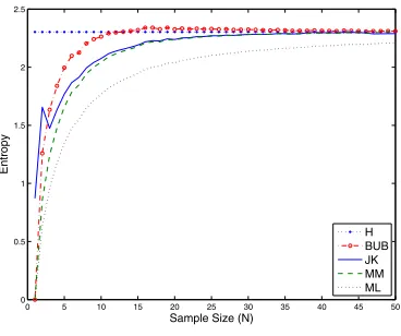
Figure 1

The estimated and true entropy for uniform distribution.

the estimates (and their biases) with the true entropy. In all our experiments, we set the number of clusters m to 10 and varied the sample size N (Figure 1). Each point on the graph is the result of averaging over 1,000 sampling experiments.6

The distribution of senses for a given word is normally skewed: For most words the vast majority of occurrences correspond to one or two most common senses even though the total number of senses can be quite large (Kilgarriff 2004). This type of long-tail distribution can be modeled with Zipf’s law. Consequently, most of our experiments consider Zipfian distributions. For Zipf’s law, the probability of choosing an element with rank k is proportional to 1

ks, where s is a shape parameter. Small values of the

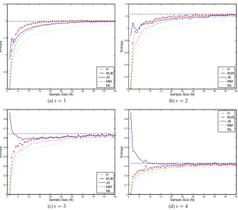
parameter s correspond to flatter distributions; the distributions with a larger s are increasingly more skewed. The estimators’ prediction for Zipfian distributions with a different s are shown in Figure 2. For s=4, over 90% of the probability mass is concentrated on a single class. For every distribution we plot the true entropy (H) and the estimated values; compare results with a uniform distribution as seen in Figure 1.

In all figures, we observe that over the entire range of sample sizes, the bias for the bias-corrected estimates is indeed reduced substantially with respect to that of the ML estimator. This difference is particularly large for smaller N—the realistic setting for the computation of H(c, k) for the WSI task. For the uniform distribution and flatter Zipf distributions (s=1 and 2), the JK estimator seems preferable for all but the smallest sample sizes (N>3). The BUB estimator outperforms the JK estimator with very skewed distributions (s=3 and s=4) and in most cases provides the least biased estimates with very small N. However, these results with very small sample sizes (N≤2) may not have much practical relevance as any estimator is highly inaccurate in this mode. The MM bias correction, as expected, is not sufficient for small N. Although it outperforms the ML estimates, its error is consistently larger than those of other bias-correction strategies.

Overall, the simulations suggest that the ML estimators are not very appropriate for entropy estimation with the types of distributions which are likely to be observed in the

0 5 10 15 20 25 30 35 40 45 50 0 0.5 1 1.5 2 2.5

Sample Size (N)

Entropy H BUB JK MM ML

0 5 10 15 20 25 30 35 40 45 50 0 0.2 0.4 0.6 0.8 1 1.2 1.4

Sample Size (N)

Entropy H BUB JK MM ML

(a)s=1 (b)s=2

0 5 10 15 20 25 30 35 40 45 50 0 0.1 0.2 0.3 0.4 0.5 0.6 0.7 0.8 0.9

Sample Size (N)

Entropy H BUB JK MM ML

0 5 10 15 20 25 30 35 40 45 50 0 0.1 0.2 0.3 0.4 0.5 0.6 0.7 0.8 0.9

Sample Size (N)

Entropy H BUB JK MM ML

(c)s=3 (d)s=4

Figure 2

The estimated and true entropy of Zipf’s law.

WSI tasks. Both the JK and BUB estimators are considerably less biased alternatives to the ML estimations.

5. Effects on WSI Evaluation

To gauge the effect of the bias problem on WSI evaluation, we computed how the ranking of the SemEval 2010 systems (Manandhar et al. 2010) were affected by different estimators. The SemEval 2010 organizers supplied a test set containing 8,915 manually annotated examples covering 100 polysemous lemmas.

The average number of gold standard senses per lemma was 3.79. Overall, 27 systems participated and were ranked according to their performance on the test set, applying the V-measure evaluation as well as paired F-score and a supervised evaluation scheme. The systems were also compared against three baselines. For the Most Frequent Sense (MFS) baseline all test instances of a given target lemma are grouped into one cluster, that is, there is exactly one cluster per lemma. The second baseline, Random, assigns each instance randomly to one of four clusters. The last baseline, proposed in Manandhar and Klapaftis (2009), 1-cluster-per-instance (1ClI), produces as many clusters as there are instances in the test set.

Table 1

V-measure computed with different estimators. Supervised recall is shown for comparison (80:20 and 60:40 splits for mapping/evaluation, numbers as provided by Manandhar et al. 2010). The corresponding ranks are shown in parentheses.

System C# ML MM JK BUB Supervised Recall

80:20 60:40

1ClI 89.1 31.6 (1) 29.5 (1) 27.4 (1) –3.6 (29) – –

Hermit 10.8 16.2 (2) 13.1 (4) 10.7 (4) 11.0 (2) 58.3 (17) 57.3 (18)

UoY 11.5 15.7 (4) 14.3 (2) 13.1 (2) 11.4 (1) 62.4 (1) 62.0 (1)

KSU KDD 17.5 15.7 (3) 13.2 (3) 11.0 (3) 7.6 (3) 52.2 (24) 50.4 (25)

Duluth-WSI 4.1 9.0 (5) 6.9 (5) 5.7 (5) 5.6 (5) 60.5 (2) 59.5 (5)

Duluth-WSI-SVD 4.1 9.0 (6) 6.9 (6) 5.7 (6) 5.6 (6) 60.5 (3) 59.5 (4)

Duluth-R-110 9.7 8.6 (7) 4.7 (16) 1.9 (20) 3 (17) 54.8 (23) 53.6 (23)

Duluth-WSI-Co 2.5 7.9 (8) 6.4 (7) 5.7 (7) 5.7 (4) 60.8 (4) 60.1 (2)

KCDC-PCGD 2.9 7.8 (9) 6.3 (8) 5.5 (8) 5.2 (7) 59.5 (9) 59.1 (7)

KCDC-PC 2.9 7.5 (10) 6.2 (9) 5.4 (9) 5.0 (8) 59.7 (8) 58.9 (9)

KCDC-PC-2 2.9 7.1 (11) 5.7 (12) 4.9 (12) 4.5 (13) 59.8 (7) 58.9 (8)

Duluth-Mix-Narrow-Gap 2.4 6.9 (15) 5.5 (14) 4.8 (14) 4.8 (9) 56.6 (21) 56.2 (21)

KCDC-GD-2 2.8 6.9 (14) 5.7 (11) 4.9 (11) 4.6 (12) 58.7 (13) 57.9 (15)

KCDC-GD 2.8 6.9 (12) 5.8 (10) 5.0 (10) 4.6 (11) 59.0 (11) 58.3 (11)

Duluth-Mix-Narrow-PK2 2.7 6.8 (16) 5.4 (15) 4.6 (15) 4.6 (10) 56.1 (22) 55.7 (22)

Duluth-MIX-PK2 2.7 5.6 (17) 4.3 (17) 3.5 (17) 3.5 (16) 51.6 (25) 50.5 (24)

Duluth-R-15 5.0 5.3 (18) 2.4 (20) 0.7 (24) 1.3 (22) 56.8 (20) 56.5 (19)

Duluth-WSI-Co-Gap 1.6 4.8 (19) 4.1 (18) 3.8 (16) 4.1 (15) 60.3 (5) 59.5 (3)

Random 4.0 4.4 (20) 1.9 (22) 0.5 (25) 0.8 (24) 57.3 (19) 56.5 (20)

Duluth-R-13 3.0 3.6 (21) 1.5 (25) 0.5 (26) 0.7 (25) 58.0 (18) 57.6 (17)

Duluth-WSI-Gap 1.4 3.1 (22) 2.6 (19) 2.5 (18) 2.7 (18) 59.8 (6) 59.3 (6)

Duluth-Mix-Gap 1.6 3.0 (23) 2.3 (21) 1.9 (19) 2.0 (19) 50.6 (26) 49.8 (26)

Duluth-Mix-Uni-PK2 2.0 2.4 (24) 1.8 (23) 1.5 (21) 1.4 (21) 19.3 (27) 19.1 (27)

Duluth-R-12 2.0 2.3 (25) 0.8 (27) 0.2 (27) 0.3 (28) 58.5 (16) 57.7 (16)

KCDC-PT 1.5 1.9 (26) 1.6 (24) 1.4 (22) 1.5 (20) 58.9 (12) 58.3 (13)

Duluth-Mix-Uni-Gap 1.4 1.4 (27) 1.0 (26) 0.8 (23) 1.0 (23) 18.7 (28) 18.9 (28)

KCDC-GDC 2.8 6.9 (13) 5.7 (13) 4.8 (13) 4.5 (14) 59.1 (10) 58.3 (10)

MFS 1.0 0 (29) 0.0 (29) 0.0 (28) 0.5 (27) 58.7 (15) 58.3 (12)

Duluth-WSI-SVD-Gap 1.0 0.0 (28) 0.0 (28) 0.0 (29) 0.5 (26) 58.7 (14) 58.2 (14)

KCDC-PC-2* 2.9 5.7 7.2 2.3 2.2 – –

UoY* 11.5 25.1 22.8 17.8 5.0 – –

SemEval 2010 results table (Table 4 in Manandhar et al. (2010), p. 66). Table 1 shows the average number of clusters per word (C#), the V-measure computed with different estimators (ML, MM, JK, and BUB), and the rankings it produces (in brackets).7 _For comparison, the results of a supervised evaluation are also shown. The bottom two rows (KCDC-PC-2∗ and UoY∗) show the scores computed from the stochastic (weighted) output (Section 3.3) for systems KCDC-PC-2 and UoY, respectively. Other systems did not produce weighted output.

0 2 4 6 8 10 12 14 16 18 0

0.01 0.02 0.03 0.04 0.05 0.06 0.07

Average Cluster Number

ML−JK

0 2 4 6 8 10 12 14 16 18

−0.01 0 0.01 0.02 0.03 0.04 0.05 0.06 0.07 0.08 0.09

Average Cluster Number

ML−BUB

(a) ˆH - ˆHJK (b) ˆH - ˆHBUB

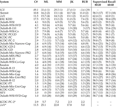
Figure 3

Discrepancy in estimates as a function of the predicted number of classes.

The 27 systems vary widely in the number of average clusters they output per lemma, ranging from 1.02 (Duluth-WSI-SVD) to 17.5 (KSU-KDD). To assess the influence of the cluster granularity on the entropy estimates, we compared the estimates given by the ML estimator against those given by JK and BUB for different numbers of clusters. Figure 3 plots the cluster numbers output by the systems against the estimate difference for ML vs. JK (Figure 3a) and ML vs. BUB (Figure 3b). If two estimators agree perfectly (i.e., produce the same estimate), their difference should always be zero, independent of the number of clusters. As can be seen, this is not the case. As expected, the difference is larger for systems with larger numbers of clusters, such as KSU-KDD. This trend will result in unfair preference towards systems producing richer clusterings.

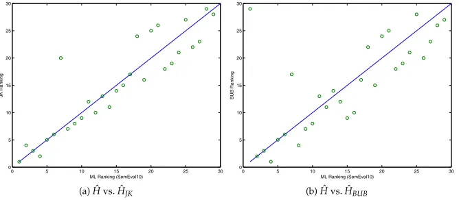
Figure 4 shows the effect that the discrepancy in estimates has on the rankings produced by using either of the three estimators. Figure 4a plots the ranking of the ML estimator against JK, and Figure 4b plots the ranking of ML against BUB. Dots that lie on the diagonal line indicate systems whose rank has not changed. It can be seen that this only applies to a minority of the systems. In general, there are significant differences between the rankings produced by ML and those by JK or BUB. We have seen that the ML estimator can lead to counterintuitive and undesirable results, such as ranking the

0 5 10 15 20 25 30

0 5 10 15 20 25 30

ML Ranking (SemEval10)

JK Ranking

0 5 10 15 20 25 30

0 5 10 15 20 25 30

ML Ranking (SemEval10)

BUB Ranking

(a) ˆH vs. ˆHJK (b) ˆH vs. ˆHBUB

Figure 4

1-cluster-per-instance baseline highest. The BUB estimator corrects this and assigns the last rank to this baseline.8

The estimate for the V-measure is based on the estimates of the marginal and joint entropies. To confirm our intuition that joint entropies are more significantly corrected, we looked into the differences between estimates of each entropy for five systems with the largest number of clusters (excluding the 1C1I baseline). The average differences in estimation of H(k) and H(k, c) between JK and ML estimators are 0.08 and 0.16, respectively, confirming our hypothesis. Analogous discrepancies for the pair BUB vs. ML are 0.15 and 0.06, respectively. The differences in the entropy of the gold standard clustering, H(c), is less significant (<0.02 for both methods) as the gold standard is less fine-grained than the clusters proposed by these five systems.

For the stochastic version evaluation, we can observe that the score for the KCDC-PC-2 system is mostly decreased with respect to the “deterministic” evaluation (except for the MM estimator). Conversely, the score of UoY is mostly improved except to the prediction of the BUB estimator. These differences are somewhat surprising: The stochastic version resulted in significantly larger disagreement between the estimators than the deterministic version. We do not yet have a satisfactory explanation for this phenomenon.

It is important to notice that for the vast majority of the systems there is agreement between the scores of the JK and BUB estimator, wheres the ML estimator significantly overestimates the V-measure for most of the systems. This observation, coupled with the observed behavior of the JK and BUB estimators in the simulations, suggest that their predictions are considerably more reliable than predictions of the plug-in ML estimator.

Comparing the V-measure (BUB) rankings to those obtained by supervised evalu-ation (last two columns in Table 1) shows noticeable differences. Several systems that rank highly according to the V-measure occupy the lower end of the scale when evalu-ated according to supervised recall (Hermit, KSU KDD, Duluth-Mix-Narrow-Gap).

6. Conclusions

In this work, we analyzed the shortcomings of information-theoretic measures in the context of WSI evaluation and argued that main drawbacks of these approaches, such as the preference for the systems predicting richer clusterings or assigning the top score to the 1-cluster-per-instance baseline, are caused by the bias of the underlying sample-based estimates of entropy. We studied alternative estimators, including one specifically designed to deal with cases where the number of examples is comparable with the num-ber of clusters. Two of the considered estimators, the jackknifed estimator and the best-upper-bound estimator, achieve consistently and significantly less biased results than the standard ML estimator when evaluated in simulations with Zipfian distributions. The corresponding estimates in the WSI evaluation context can result in significant changes in scores and relative rankings, with systems producing richer clusterings more severely affected. We believe that these results strongly suggest that more accurate estimates of entropy should be used in future evaluations of sense induction systems. Other unsupervised tasks in natural language processing, such as word clustering or

named entity disambiguation, may also benefit from using information-theoretic scores based on more accurate estimators.

Appendix A: Derivation for the BUB Estimator

We provide a brief derivation for the BUB estimator and refer the reader to Paninski (2003) for details and discussion. The BUB estimator is obtained by minimizing an upper bound on MSE for estimators H(aaa) (see Equation (2)). First, MSE is bounded from above by maximizing the variance and the bias independently:

max

p Bp( ˆH(aaa))

2_+V

p( ˆH(aaa))≤max

p Bp( ˆH(aaa))

2_+max

p Vp( ˆH(aaa)) (A.1)

where p=(p1,. . ., pm) is an underlying discrete measure; Bpand Vpare the bias and the

variance of the estimator given p. Then individual bounds both for the squared bias and the variance can be constructed.

We start by deriving a bound for the bias. Using linearity of expectation, the expec-tation of ˆH(aaa) can be written as

Ep( ˆH(aaa))= N

j=0

aj,NEp(hj)= N

j=0 aj,N

m

i=1

Bj,N(pi)

where Bj,N(x) is the binomial polynomial

_N

j

xj(1−x)N−j. Then, with simple algebra, we have

Bp( ˆH(aaa))= m

i=1

⎛ ⎝N

j=0

aj,NBj,N(pi)−H(pi)

⎞ ⎠

where H(x)=−x log x, the entropy function. A uniform upper bound can be obtained by bounding each term in the sum:

|Bp( ˆH(aaa))| ≤m sup

x |

N

j=0

aj,NBj,N(x)−H(x)|

However, this bound is not too tight as it would overemphasize importance of the approximation quality for components i with piclose to 1. Intuitively, the behavior near

0 is more important, as there can be more components pi close to 0. Paninski (2003)

generalizes this bound by considering a weighted version

|Bp( ˆH(aaa))| ≤2 sup x

f (x)|

N

j=0

aj,NBj,N(x)−H(x)| (A.2)

with the function f chosen to emphasize smaller components

f (x)=

m, x< 1

m

1/x, x≥ 1

As shown in Antos and Kontoyiannis (2001) and in Paninski (2003), bounds on the variance of the estimator ˆH(aaa) can be derived using either McDiarmid or Steele bounds (Steele 1986). For the Steele bound, it has the form

Vp( ˆH(aaa))<N max

0≤j<N(aj+1−aj)

2 _(A.3)

Finally, MSE can be bounded by substituting Equations (A.2) and (A.3) into the inequality (A.1). For computational reasons, instead of choosing aaa to minimize the bound, the L2relaxation of the L∞loss is used, resulting in a regularized least-squares

problem.

Acknowledgments

The research was carried out when the authors were at Saarland University. It was funded by the German Research Foundation DFG (Cluster of Excellence on Multimodal

Computing and Interaction, Saarland

University, Germany). We would like to thank the anonymous reviewers for their valuable feedback.

References

Agirre, Eneko, David Mart´ınez, Oier L ´opez de Lacalle, and Aitor Soroa. 2006. Evaluating and optimizing the parameters of an unsupervised graph-based WSD algorithm. In Workshop on TextGraphs, at HLT-NAACL

2006, pages 89–96, New York, NY.

Agirre, Eneko and Aitor Soroa. 2007. Semeval-2007 task 02: Evaluating word sense induction and discrimination systems. In Proceedings of the 4th

International Workshop on Semantic Evaluation, pages 7–12, Prague.

Amigo, Enrique, Julio Gonzalo, Javier Artiles, and Felisa Verdejo. 2009. A comparison of extrinsic clustering evaluation metrics based on formal constraints. Information Retrieval, 12(4):461–486.

Antos, A. and I. Kontoyiannis. 2001. Convergence properties of functional estimates of discrete distributions. Random

Structures and Algorithms, 19:163–193.

Bagga, Amit and Breck Baldwin. 1998. Algorithms for scoring coreference chains. In The First International Conference on

Language Resources and Evaluation Workshop on Linguistics Coreference, pages 563–566,

Granada.

Batu, Tugkan, Sanjoy Dasgupta, Ravi Kumar, and Ronitt Rubinfeld. 2002. The complexity of approximating entropy. In Symposium

on the Theory of Computing (STOC),

pages 678–687, Montreal.

Dom, Byron E. 2001. An information-theoretic external cluster-validity measure. Technical Report No. RJ10219, IBM. Grasberger, P. and T. Sch ¨urmann. 1996.

Entropy estimation of symbol sequences.

CHAOS, 6(3):414–427.

Kilgarriff, Adam. 2004. How dominant is the commonest sense of a word? In Sojka, Kopecek, and Pala, editors, Text,

Speech, Dialogue, volume 3206 of Lecture Notes in Artificial Intelligence. Springer,

pages 103–112.

Klapaftis, Ioannis P. and Suresh Manandhar. 2013. Evaluating word sense induction and disambiguation methods. Language

Resources and Evaluation, 47(3):1–27.

Luo, Xiaoqiang. 2005. On coreference resolution performance metrics. In

Proceedings of the Conference on Human Language Technology and Empirical Methods in Natural Language Processing (HLT-05),

pages 25–32, Vancouver.

Manandhar, Suresh and Ioannis Klapaftis. 2009. Semeval-2010 task 14: Evaluation setting for word sense induction & disambiguation systems. In Proceedings of

the Workshop on Semantic Evaluations: Recent Achievements and Future Directions (SEW-2009), pages 117–122, Boulder, CO.

Manandhar, Suresh, Ioannis Klapaftis, Dmitriy Dligach, and Sameer Pradhan. 2010. Semeval-2010 task 14: Word sense induction & disambiguation. In Proceedings

of the 5th International Workshop on Semantic Evaluation, pages 63–68, Uppsala.

Meila, Marina. 2007. Comparing clusterings—an information based distance. Journal of Multivariate Analysis, 98:873–895.

Miller, G. 1955. Note on the bias of

information estimates. Information Theory

in Psychology II-B, pages 95–100.

Paninski, Liam. 2003. Estimation of entropy and mutual information. Neural

Paninski, Liam. 2004. Estimating entropy of m bins given fewer than m samples.

IEEE Transactions on Information Theory,

50(9):2,200–2,203.

Purandare, Amruta and Ted Pedersen. 2004. Word sense discrimination by clustering contexts in vector and similarity spaces. In Proceedings of the CoNLL, pages 41–48, Boston, MA.

Quenouille, M. 1956. Notes on bias and estimation. Biometrika, 43:353–360. Rosenberg, Andrew and Julia Hirschberg.

2007. V-measure: A conditional entropy-based external cluster evaluation measure. In Proceedings of the 2007

EMNLP-CoNll Joint Conference,

pages 410–420, Prague.

Sch ¨utze, Hinrich. 1998. Automatic word sense discrimination. Computational

Linguistics, 24(1):97–123.

Steele, J. Michael. 1986. An Efron-Stein inequality for nonsymmetric statistics.

Annals of Statistics, 14:753–758.

Strehl, Alexander and Joydeep Gosh. 2002. Cluster ensembles: A knowledge reuse framework for combining multiple partitions. Journal of Machine Learning

Research, 3:583–617.

Strong, S., R. Koberle, S. R. van de Ruyter, and W. Bialek. 1998. Entropy and information in neural spike trains.

Physical Review Letters, 80:197–202.

Tukey, J. 1958. Bias and confidence in not quite large samples. Annals of Mathematical

Statistics, 29:614.

Wang, Y. H. 1993. On the number of successes in independent trials. Statistica

Sinica 3, 2:295–312.

Witte, Ian and Eibe Frank. 2005. Data

Mining: Practical Machine Learning Tools and Techniques. Morgan Kaufmann,

Amsterdam.

Zhao, Y. and G. Karypis. 2005. Hierarchical clustering algorithms for document datasets. Data Mining and Knowledge