Multiple Particle Swarm Optimizers with Inertia
Weight for Multi-objective Optimization
Hong Zhang, Member, IAENG
Abstract—An improved particle swarm optimizer with inertia weight (PSOIWα) was applied to multi-objective optimization (MOO). In this paper we present a method of multiple particle swarm optimizers with inertia weight (MPSOIWα), which belongs to a kind of the methods of cooperative particle swarm optimization. The crucial idea of the MPSOIWα, here, is to reinforce the search ability of the PSOIWα by the union’s power of plural swarms. To demonstrate its effectiveness and search performance, computer experiments on a suite of 2-objective optimization problems are carried out by a weighted sum method. The resulting Pareto-optimal solution distribu-tions corresponding to each given problem indicate that the linear weighted aggregation among the adopted three kinds of dynamically weighted aggregations is the most suitable for ac-quiring better search results. Throughout quantitative analysis to experimental data, we clarify the search characteristics and performance effect of the MPSOIWαcontrast with that of the PSOIWαand MPSOIW.
Index Terms—particle swarm optimization, swarm intelli-gence, hybrid search, multi-objective optimization, weighted sum method.
I. INTRODUCTION
M
ULTI-objective optimization (MOO) is the processing of optimizing simultaneously two and more conflict-ing objectives subject to certain constraints [4], [6]. Since many practical problems are involved in MOO, which can be mainly found in different domains of science, technology, in-dustry, finance, automobile design, aeronautical engineering and so on [8], [11], [23], how to efficiently deal with MOO becomes a live issue, and is centered on the development of the treatment technique.Particle swarm optimization (PSO), which was created by Kennedy and Eberhart in 1995, is an adaptive, stochastic, and population-based optimization technique [15]. Based on the special features, i.e. information exchange, intrinsic mem-ory, and directional search, the technique has higher latent search ability in optimization compared to some methods of evolutionary computation (EC) such as genetic algorithms and genetic programming [19], [20], [26], [27]. Especially, in recent years, a large number of studies, and investigations on cooperative PSOain relation to symbiosis, group behavior, and synergy are in the researcher’s spotlight. Various kinds of the methods of cooperative PSO, for example, hybrid
Manuscript received December 30, 2011; revised January 27, 2012. This work was supported in part by Grant-in-Aid Scientific Research (C)(22500132) from the Ministry of Education, Culture, Sports, Science and Technology, Japan.
H. Zhang is with the Department of Brain Science and Engineering, Graduate School of Life Science & Systems Engineering, Kyushu Institute of Technology, 2-4 Hibikino, Wakamatsu, Kitakyushu 808-0196, Japan. phone/fax: +81-93-695-6112; e-mail: [email protected].
aCooperative PSO is generally considered as multiple swarms (or
sub-swarms) searching for a solution (serially or in parallel) and exchanging some information during the search according to some communication strategies.
PSO, multi-layer PSO, multiple PSO with decision-making strategy etc. were published [2], [10], [17], [27].
In contrast to those methods running a single particle swarm, many attempts and strategies can be perfected with operating multiple particle swarms for more efficiently find-ing an optimal solution or near-optimal solutions [3], [14], [17], [28]. Owing to the plain advantage, utilizing the tech-niques of group searching, parallel and intelligent processing has become one of extremely important approaches to opti-mization, and a lot of publications and reports have been shown that the methods of cooperative PSO have better adaptability and higher search performance than ones of uncooperative PSO in dealing with various optimization and practical problems [18].
An improved particle swarm optimizer with inertia weight (PSOIWα) was published [30]. For further upgrading its search performance to MOO, in this paper we propose to use a method of cooperative PSO, called multiple particle swarm optimizers with inertia weight (MPSOIWα). The crucial idea of the MPSOIWα, here, is to reinforce the search ability of the PSOIWα by the union’s power of plural swarms. Although the search feature and performance of some PSO methods in MOO with fitness assignment manners such as criterion-based manner or dominance-based manner were studied and investigated [24], [25], there are insufficient results for systematically solving MOO problems by an aggregation-based manner, and analyzing the potential characteristics in details from the obtained experimental results [6], [16].
To demonstrate the effectiveness and performance ef-fect of the MPSOIWα, computer experiments on a suite of 2-objective optimization problems are carried out by a weighted sum method. For interpreting the information treat-ment and search effect of the method, we show the distribu-tions of the obtained Pareto-optimal soludistribu-tions corresponding to each given problem by respectively using three kinds of dynamically weighted aggregations (i.e. linear weighted aggregation, bang-bang weighted aggregation, and sinusoidal weighted aggregationb), point out that which one of them is the most suitable for acquiring good search results to the given MOO problems, and clarify the search characteristics and performance of the MPSOIWαcontrast with that of the PSOIWαand MPSOIW.
II. BASICCONCEPTS
For explaining how to treat with MOO by a fitness assignment manner, some basic concepts and definitions on a general MOO problem, Pareto-optimal solution, front distance, cover rate, a weighted sum method, and three kinds of dynamically weighted aggregations are briefly described.
bMany researchers call sinusoidal weighted aggregation (SWA) as
A. MOO Problem
In general, the formulation of a MOO problem can be defined as follows.
M inimize
~
x f1(~x), f2(~x),· · ·, fI(~x)
T
s.t. gj(~x)≥0, j= 1,2,· · ·, J
hm(~x) = 0, m= 1,2,· · ·, M xn∈[xnl, xnu], n∈(1,2,· · ·, N)
(1)
where fi(~x) is the i-th objective, gj(~x) is the j-th in-equality constraint, hm(~x) is the m-th equality constraint,
~x = (x1, x2,· · ·, xN)T ∈ <N = Ω (search space) is the
vector of decision variable, xnl and xnu are the superior
boundary value and the inferior boundary value of each component xn of the vector~x, respectively.
Due to the given condition ofI≥2, theI-objectives may be conflicting with each other. Under this circumstance, it is difficult to obtain the global optimum corresponding to each objective by traditional optimization methods at the same time. Consequently, the goal of handling the MOO problem is effectively to achieve a set of solutions that satisfy Pareto optimality for improvement of mental capacity.
B. Pareto-optimal Solution
A solution ~x∗ ∈Ω is said to be Pareto-optimal solution
if and only if there does not exist another solution~x∈Ωso thatfi(~x)is dominated byfi(~x∗). The formula of the above relationship is expressed as
fi(~x)6≤fi(~x∗) ∀i∈I iif fi(~x)6< fi(~x∗) ∃i∈I (2)
In other words, this definition says that ~x∗ is a
Pareto-optimal solution if there exists no feasible solution (vector)
~x which would decrease some criteria without causing a simultaneous increase in at least one other criterion.
Furthermore, all the Pareto-optimal solutions for a given MOO problem are composed of the Pareto-optimal solution set (P∗), or the Pareto front (P F).
C. Weighted Sum Method
There are some fitness assignment manners such as aggregation-based one, criterion-based one, and dominance-based one, which are used for MOO [7], [12]. As to be gen-erally known, a conventional weighted sum (CWS) method is a straightforward approach applied to deal with MOO problems. In this case, the different objectives are summed up to a single scalar Fs (criterion) with some prescribed weights as follows.
Fs(~x) =
I
X
i=1
cifi(~x) (3)
whereci(i= 1,2,· · ·, I) is the non-negative weight. During the optimization, usually, these weights are fixed by the constraint of PIi=1ci = 1, and prior knowledge is also needed to specify these weights for obtaining good solutions. To thoroughly conquer the weakness of the CWS method run, the following dynamically weighted sum (DWS) method is often used to MOO in practice. The criterion Fd of the method can be expressed as follows.
Fd(t, ~x) =
I
X
i=1
ci(t)fi(~x) (4)
where t is time-step to search, and ci(t) ≥ 0 is the
dy-namic weight. In order to present the method, a 2-objective optimization problem is considered as an example. Hence, the definitions of three kinds of the adopted dynamically weighted aggregations are expressed below.
• Linear weighted aggregation (LWA):
c1l(t) =mod t
T,1
, cl2(t) = 1−c1l(t)
• Bang-bang weighted aggregation (BWA):
c1b(t) =
sign sin(2π t/T)+1
2 , c
b
2(t) = 1−c1b(t)
• Sinusoidal weighted aggregation (SWA):
c1s(t) = sin π t
T
, c2s(t) = 1−c1s(t)
where T is a period of the variable weights in the above equations.
D. Front Distance
Front distance is expressed as a metric of checking how far the elements are in the set of non-dominated solutions found from those in the true Pareto-optimal solution set. It directly reflects the estimation accuracy of the optimizer used. Concretely, the definition of front distance (F D) is expressed as
F D= 1
Q v u u tXQ
q=1 d2
q, dq =fi(~xq∗)−fi(~xqo), ∀i∈I (5)
where Q is the number of the elements in the set of non-dominated solutions found, anddq is the Euclidean distance
(measured in objective space) between each of these obtained optimal solutions,~xo, and the nearest member,~x∗, of the true Pareto-optimal solution set.
E. Cover Rate
Cover rate (CR) is an other metric for checking the coverage of the elements being in the set of non-dominated solutions found to the Pareto front. This is because the estimation accuracy is insufficiency to reveal the distribution status of the obtained Perato-optimal solutions and their possibility for dealing with the given problem.
Here, the formulation of CR is mathematically expressed by
CR= 1
I
I
X
i=1
CRi (6)
whereCRiis the partial cover rate corresponding to thei-th objective, which is defined as
CRi=
PΓ
l=1γl
Γ (7)
whereΓ is the number of dividing the i-th objective space which is from the minimum to the maximum of the fitness value, i.e.[fi(~x)min, fi(~x)max], andγl∈(0,1)indicates the
III. ALGORITHMS
For the convenience of the following description to the used every optimizer, let the search space beN-dimensional, the number of particles of a swarm beP, the position of the
i-th particle be~xi= (x1i, x2i,· · ·, xiN)T ∈Ω, and its velocity be~vi= (v1i, v2i,· · ·, vNi )T ∈Ω, respectively.
A. The PSOIW
To overcome the weak convergence of the original PSO [1], [5], Shi et al. modified the update rule of the i-th parti-cle’s velocity by constant reduction of the inertia coefficient over time-step [9], [21]. Concretely, the formulation of the particle swarm optimizer with inertia weight (PSOIW) is defined as
( ~xi
k+1=~xki +~vki+1 ~vi
k+1=w(k)~vki+w1~r1⊗(~pki−~xki) +w2~r2⊗(~qk−~xki)
(8)
wherew1 andw2 are coefficients for individual confidence and swarm confidence, respectively.~r1,~r2∈ <N are two ran-dom vectors, each element of which is uniformly distributed on the interval [0,1], and the symbol ⊗is an element-wise operator for vector multiplication.~pi
k(=arg maxk=1,2,···{g(~xki)},
whereg(~xi
k)is the criterion value of thei-th particle at
time-stepk) is the local best position of thei-th particle up to now,
~qk(=arg max
i=1,2,···{g(~p
i
k)})is the global best position among
the whole particles at time-step k. w(k) is the following variable inertia weight which is linearly reduced from a starting valuews to a terminal valuewe with the increment
of time-step k.
w(k) =ws+
we−ws
K ×k (9)
whereK is the number of iteration for the PSOIW run. In the original PSOIW, two terminal values,wsandwe, are set
to 0.9 and 0.4, respectively, andw1=w2= 2.0 are used as
same as the original PSO.
Owing to the bigger difference between the two boundary values of the variable inertia weight, it is obvious that the search behavior of the PSOIW achieves a search shift which smoothly changes from exploratory mode to exploitative one in the whole optimization process. Hence, this way is very simple and useful for conquering the weakness of the PSO in convergence and enhancing the solution accuracy. On the other hand, the shortcoming of the PSOIW is easily to fall into a local minimum and hardly to escape from that place in dealing with multimodal problems because the terminal valuewe is set to small.
B. The PSOIWα
For alleviating the weakness of the PSOIW search, we introduce the LRS [22], [29] into the PSOIW to form a hybrid search optimizer (called PSOIWα). Implementing the PSOIWα, here, is to enable a particle swarm search escapes from local minimum sooner for efficiently obtaining an optimal solution or near-optimal solutions.
The PSOIWα’s procedure is implemented as follows.
step-1: Give the terminating condition, U (the number of random data) of the PSOIWα run, and set the counteru= 1.
step-2: Implement PSOIW and determine the best solu-tion~qk at time-stepk, and set~qnow=~qk. step-3: Generate a random data, ~zu ∈ <N ∼N(0, σ2)
(where σ is a small positive value given by user, which determines the small limited space). Check whether~qk+~zu∈Ωis satisfied or not. If~qk+~zu6∈
Ωthen adjust~zufor moving~qk+~zuto the nearest
valid point withinΩ. Set ~qnew=~qk+~zu.
step-4: Ifg(~qnew)> g(~qnow)then set~qnow=~qnew.
step-5: Setu=u+ 1. Ifu≤U then go to the step-2. step-6: Set ~qk =~qnow to correct the solution found by
the particle swarm at time-stepk. Stop the search.
C. The MPSOIWα
[image:3.595.304.549.315.526.2]For improving the search ability of the existent PSOIWα to MOO, we propose to use multiple particle swarm opti-mizers with inertial weight, MPSOIWα. Figure 1 illustrates a flowchart of the MPSOIWα.
Fig. 1. A flowchart of the MPSOIWα.
The most difference between the PSOIWαand MPSOIWα
in composition is just to implement the plural PSOIWα(S≥
2) in parallel for finding the most suitable solution or near-optimal solutions. Concretely, the best solution of the multi-swarm search, i.e.~xo
k =arg maxi=1,2,···,S{g(~qki)}, is determined
from the solutions obtained by each PSOIWα run at time-stepk, and then put it into a solution set which is the storage memory of the multi-swarm.
It is obvious that the MPSOIWα is the use of swarm intelligence to search by the union’s power of plural swarms for enforcing the search ability of the PSOIWα. It is to be noted that if the LRS is not implemented after each PSOIW run, the method will be called as MPSOIW.
IV. COMPUTEREXPERIMENTS
TABLE I
ASUITE OF2-OBJECTIVE OPTIMIZATION PROBLEMS
problem objective search range
ZDT1 f11(~x) =x1, g(~x) = 1 +
9
N−1
N X
n=2
xn, f12(~x) =g(~x)
1−
r f11(~x)
g(~x)
Ω∈[0,1]N
ZDT2 f21(~x) =x1, f22(~x) =g(~x) 1−
f21(~x) g(~x)
2!
Ω∈[0,1]N
ZDT3 f31(~x) =x1, f32(~x) =g(~x)
1−
r f31(~x)
g(~x) −
f31(~x)
g(~x)
sin 10πf31(~x)
Ω∈[0,1]N
Fig. 2. Solution distributions of the MPSOIWαand MPSOIW by using the LWA (red-point), BWA (blue-point) and SWA (green-point), respectively. Notice: the distance between the experimental data sets for each subgraph is 0.05 (shift only in horizontal direction).
optimization problems [31] in Table I is used in the next com-puter experiments. The characteristics of the Pareto fronts of the given problems include the convex (ZDT1), concave (ZDT2), and discontinuous multimodal (ZDT3), respectively.
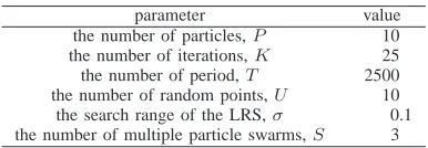
TABLE II
MAJOR PARAMETERS OF THEMPSOIWαRUN
parameter value
the number of particles,P 10 the number of iterations,K 25 the number of period,T 2500 the number of random points,U 10 the search range of the LRS,σ 0.1 the number of multiple particle swarms,S 3
Table II gives the major parameters of the MPSOIWα for solving the given problems in Table I. The choice of
their values is referred to the results of some preliminary experiments.
A. Performance Comparison
For the sake of observation, Figure 2 shows the resulting solution distributions of the MPSOIWα and MPSOIW by using the LWA, BWA, and SWA, respectively. According to the distinction of each solution distribution corresponding to these given problems, the analytical judgment can be described as follows.
1) Regardless of the used methods either the MPSOIWα
TABLE III
PERFORMANCE COMPARISON OF BOTH THEMPSOIWαANDMPSOIWBY USING THELWA, BWA,ANDSWA,RESPECTIVELY(ΓIS SET TO100).
MPSOIWα MPSOIW
problem aggregation solution FD CR (%) solution FD CR (%)
LWA 1254 2.234×10⁻⁸ 99.5 1191 3.948×10⁻⁸ 99.5
ZDT1 BWA 187 9.809×10⁻⁵ 52.0 227 1.107×10⁻⁴ 53.0
SWA 988 4.511×10⁻⁸ 99.5 1016 7.355×10⁻⁸ 99.0
LWA 272 1.198×10⁻⁸ 94.0 283 1.992×10⁻⁷ 94.0
ZDT2 BWA 259 3.692×10⁻⁷ 92.0 228 8.852×10⁻⁷ 91.5
SWA 229 7.604×10⁻⁸ 93.5 219 3.381×10⁻⁷ 93.0
LWA 1231 8.961×10⁻⁷ 46.0 1107 9.245×10⁻⁷ 45.5
ZDT3 BWA 396 1.655×10⁻⁴ 40.5 421 6.551×10⁻⁵ 40.0
SWA 949 9.433×10⁻⁷ 42.5 1018 1.092×10⁻⁶ 42.0 # The values in bold signify the best result for each given problem.
2) Regardless of the used methods and the characteris-tics of the given problems, the conditions of solution distributions by using the BWA are worse than that by using the LWA or SWA special for the ZDT1 and ZDT3 problems.
3) In comparison with the solution distributions of using the LWA for both the ZDT1 (convex) and ZDT2 (con-cave) problems, the former is relatively in the higher density.
For quantitative analysis to the experimental results of the MPSOIWα and MPSOIW in Figure 2, Table III gives the statistical data, i.e. the number of the obtained optimal solutions ~xo, and the corresponding FD and CR for each
given problem.
The following features can be observed from Table III. Firstly, there is the most number of solutions obtained by using the LWA for the given problems even for the ZDT2 one in where a large number of Pareto-optimal solutions are in unstable position [13]. Secondly, the solution accuracy of the MPSOIWα is superior to that of the MPSOIW for each given problem. Thirdly, the obtained results of using the LWA in CR index are the best than that of using BWA and SWA, respectively. Fourthly, the search performance of using the LWA is not only much better than that of using the BWA, but also is relatively better than that of using the SWA as a whole.
Therefore, the effectiveness and search ability of the MPSOIWα are roughly confirmed by the above analytical results. Furthermore, better solution distribution and higher solution accuracy can be observed as well by using either the LWA or SWA. Our experimental results indicate that smooth change of their criteria with the growth of time-step t can make that the probability finding good solutions greatly goes up in the same period, T=2500, as evidence.
Based on the above mentioned comparison and observa-tion, the relationship of domination reflecting the search per-formance (SP) of the MPSOIWαby using each dynamically weighted aggregation can be expressed as follows.
SPLW ASPSW ASPBW A
The relationship of the above domination indicates that the uniform change of the weights can make the moving process of variable criterion to be equalization which raises the probability finding the Perato-optimal solution to the maximum under the condition of implementing the same optimizer. Due to this reason, more good solutions can be easily obtained during the short search cycle, K= 25.
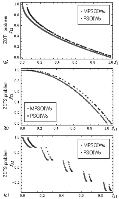
B. Effect of Multi-swarm Search
For equal treatment in search, the number of particles used in a swarm is the same to the total number of particles used in the 3-swarms. As an example, Figure 3 shows the resulting solution distributions of both the MPSOIWα and PSOIWα
[image:5.595.324.518.330.655.2](i.e.P= 30) by using the LWA. We can see that the density of solution distributions of the MPSOIWα are higher than that of the PSOIWαfor each given problem.
Fig. 3. The solution distributions of the MPSOIWα (red-point) and PSOIWα(blue-point) by using the LWA.
Table IV gives the performance indexes, i.e. the number of the optimal solutions ~xo obtained by using the LWA,
TABLE IV
SEARCHPERFORMANCE OF BOTH THEMPSOIWαANDPSOIWα
(P= 30)BY USING THELWA (ΓIS SET TO100).
problem method solution FD CR (%)
MPSOIWα 1254 2.234×10⁻⁸ 99.5
ZDT1 PSOIWα 522 6.661×10⁻⁸ 91.0 MPSOIWα 272 1.198×10⁻⁸ 94.0
ZDT2 PSOIWα 231 9.938×10⁻⁸ 61.5 MPSOIWα 1231 8.961×10⁻⁷ 46.0
ZDT3 PSOIWα 432 4.496×10⁻⁶ 41.0
used. It is demonstrated that the MPSOIWα is a powerful method of cooperative PSO to MOO.
V. CONCLUSIONS
In this paper, multiple particle swarm optimizers with inertia weight, MPSOIWα, has been presented to MOO. Based on the composition of the MPSOIWα, it is the most simple expansion of the existent PSOIWα, which has the advantages of a hybrid search with easy-to-operation as a method of cooperative PSO.
Applications of the MPSOIWα to the given suite of 2-objective optimization problems well demonstrated its ef-fectiveness by the aggregation-based manner. Owing to the resulting experimental data by respectively using three kinds of dynamically weighted aggregations, it is observed that the search performance of the MPSOIWα is superior to that of the PSOIWα and MPSOIW, and the comparative analysis of the MPSOIWαshows that the search performance of using the LWA is better than that of using the BWA or SWA for the given MOO problems. Therefore, it is no exaggeration to say that our experimental results could offer an important evidence, i.e. choosing the dynamically weighted sum method with the LWA for efficiently dealing with complex MOO problems.
It is left for further study to apply the MPSOIWαto MOO problems in the real-world. Furthermore, in order to enhance the adaptability, efficiency, and solution accuracy of the MPSOIWα, the search strategies and attempts on prediction, intelligent and powerful cooperative PSO algorithms [2], [10], [30] will be discussed for MOO in near future.
REFERENCES
[1] F. van den Bergh, “An Analysis of Particle Swarm Optimizers,” Ph.D
thesis, University of Pretoria, Pretoria, South Africa, 2002.
[2] F. van den Bergh and A. P. Engelbrecht, “A cooperative approach to particle swarm optimization,” IEEE Transactions on Evolutionary
Computation, vol.8, Issue 3, pp.225-239, 2004.
[3] J. F. Chang, S. C. Chu, J. F. Roddick and J. S. Pan, “A parallel particle swarm optimization algorithm with communication strategies,” Journal
of information science and engineering, no.21, pp.809-818, 2005. [4] A. Chinchuluun and P. M. Pardalos, “A survey of recent developments
in multiobjective optimization,” Ann Oper Res, vol.154, pp.29-50, 2007.
[5] M. Clerc and J. Kennedy, “The particle swarm-explosion, stability, and convergence in a multidimensional complex space,” IEEE Transactions
on Evolutionary Computation, vol.6, no.1, pp.58-73, 2000.
[6] C. A. Coello Coello and M. S. Lechuga, “MOPSO: A proposal for multiple objective particle swarm optimization,” Proceedings of
Congress Evolutionary Computation (CEC’2002), vol.1, pp.1051-1056, Honolulu, HI, USA, 2002.
[7] K. Deb, Multi-Objective Optimization using Evolutionary Algorithms, John Wiley & Sons, Ltd, New York, 2001.
[8] K. Deb, “Multi-Objective Optimization,” in E. K. Burke et al. (Eds.),
Search Methodologies — Introductory Tutorials in Optimization and Decision Support Techniques, Springer, 2005.
[9] R. C. Eberhart and Y. Shi, “Comparing inertia weights and constriction factors in particleswarm optimization,” Proceedings of the 2000 IEEE
Congress on Evolutionary Computation, vol.1, pp.84-88, La Jolla, CA,
USA, 2000.
[10] M. El-Abd and M. S. Kamel, “A Taxonomy of Cooperative Particle Swarm Optimizers,” International Journal of Computational
Intelli-gence Research, ISSN 0973-1873, vol.4, no.2, pp.137-144, 2008. [11] C. R. Hema, M. P. Paulraj, R. Nagarajan, S. Yaacob, and A. H. Adom,
“Application of Particle Swarm Optimization for EEG Signal Classifi-cation,” Biomedical Soft Computing and Human Sciences, vol.13, no.1, pp.79-84, 2008.
[12] E. J. Hughes, “Multiobjective Problem Solving from Nature,” Natural
Computing Series, Part IV, pp.307-329, 2008.
[13] Y. Jin, M. Olhofer and B. Sendhoff, “Dynamic Weighted Aggregation for Evolutionary Multi-Objective Optimization: Why Does It Work and How?” Proceedings of the Genetic and Evolutionary Computation
Conference (GECCO2001), pp.1042-1049, San Francisco, CA, USA,
2001.
[14] C.-F. Juang, “A Hybrid of Genetic Algorithm and Particle Swarm Optimization for Recurrent Network Design,” IEEE Transactions on
Systems, Man and Cybernetics, Part B, vol.34, no.2, pp.997-1006, 2004. [15] J. Kennedy and R. C. Eberhart, “Particle swarm optimization,”
Pro-ceedings of the 1995 IEEE International Conference on Neural Net-works, pp.1942-1948, Piscataway, NJ, USA, 1995.
[16] X. Li, J. Branke and M. Kirley. “On Performance Metrics and Particle Swarm Methods for Dynamic Multiobjective Optimization Problems,”
Proceedings of IEEE Congress of Evolutionary Computation (CEC),
pp.1635-1643, Singapore, 2007.
[17] B. Niu, Y. Zhu and X. He, “Multi-population Cooperation Particle Swarm Optimization,” in M. Capcarrere et al. (Eds.), Advances in
Artificial Life, LNCS 3630, Springer Heidelberg, pp.874-883, 2005. [18] H. Piao, Z. Wang and H. Zhang, “Cooperative-PSO-based PID neural
network integral control strategy and simulation research with asyn-chronous motor controller design,” Journal of WSEAS Transactions on
Circuits and System, vol.8, Issue 8, pp.696-708, 2009.
[19] R. Poli, J. Kennedy and T. Blackwell, “Particle swarm optimization — An overview,” Swarm Intell, vol.1, pp.33-57, 2007.
[20] M. Reyes-Sierra and C. A. Coello Coello, “Multi-Objective Particle Swarm Optimizers: A Survey of the State-of-the-Art,” International
Journal of Computational Intelligence Research, vol.2, no.3,
pp.287-308, 2006.
[21] Y. Shi and R. C. Eberhart, “A modified particle swarm optimiser,”
Proceedings of the IEEE International Conference on Evolutionary Computation, pp.69-73, Anchorage, Alaska, USA, 1998.
[22] F. J. Solis and R. J.-B. Wets, “Minimization by Random Search Techniques,” Mathematics of Operations Research, vol.6, no.1, pp.19-30, 1981.
[23] S. Suzuki, “Application of Multi-objective Optimization and Game Theory to Aircraft Flight Control Problem”, Institute of Systems,
Control and Information Engineers, vol.41, no.12, pp.508-513, 1997
(in Japanese).
[24] P. K. Tripathi, S. Bandyopadhyay and S. K. Pal, “Multi-Objective Particle Swarm Optimization with time variant inertia and acceleration coefficient,” Information Sciences 177, pp.5033-5049, 2007.
[25] C.-S. Tsou, S.-C. Chang and P.-W. Lai, “Using Crowing Distance to Improve Multi-Objective PSO with Local Search,” in Felix T. S. Chan et al. (Eds.), Swarm Intelligence: Focus on Ant and Particle Swarm
Optimization, pp.77-86, 2007.
[26] H. Zhang and M. Ishikawa, “Evolutionary Particle Swarm Opti-mization (EPSO) – Estimation of Optimal PSO Parameters by GA,”
Proceedings of the IAENG International MultiConference of Engineers and Computer Scientists 2007 (IMECS2007), vol.1, pp.13-18, Hong
Kong, China, 2007.
[27] H. Zhang and M. Ishikawa, “Characterization of particle swarm optimization with diversive curiosity,” Journal of Neural Computing
& Applications, pp.409-415, Springer London, 2009.
[28] H. Zhang and M. Ishikawa, “The performance verification of an evolutionary canonical particle swarm optimizers,” Neural Networks, vol.23, no.4, pp.510-516, 2010.
[29] H. Zhang and J. Zhang, “The Performance Measurement of a Canon-ical Particle Swarm Optimizer with Diversive Curiosity,” Proceedings
of International Conference on Swarm Intelligence (ICSI’2010), LNCS
6145, Part I, pp.19-26, Beijing, China, 2010.
[30] H. Zhang, “Multiple Particle Swarm Optimizers with Inertia Weight with Diversive Curiosity and Its Performance Test,” IAENG
Interna-tional Journal of Computer Science, vol.38, no.2, pp.134-145, 2011. [31] E. Zitzler, K. Deb and L. Thiele, “Comparison of Multiobjective