Asynchronous and Parallel Distributed Pose Graph Optimization

Asynchronous and Parallel Distributed Pose Graph Optimization

Yulun Tian

1

, Alec Koppel

2

, Amrit Singh Bedi

2

, and Jonathan P. How

1

Abstract— We present Asynchronous Stochastic Parallel Pose Graph Optimization (ASAPP), the first asynchronous algo-rithm for distributed pose graph optimization (PGO) in multi-robot simultaneous localization and mapping (SLAM). By enabling robots to optimize their local trajectory estimates without synchronization, ASAPP offers resiliency against com-munication delays and alleviates the need to wait for stragglers in the network. Furthermore, the same algorithm can be used to solve the so-called rank-restricted semidefinite relaxations of PGO, a crucial class of non-convex Riemannian optimization problems at the center of recent PGO solvers with global optimality guarantees. Under bounded delay, we establish the global first-order convergence of ASAPP using a sufficiently small stepsize. The derived stepsize depends on the worst-case delay and inherent problem sparsity, and furthermore matches known result for synchronous algorithms when there is no delay. Numerical evaluations on both simulated and real-world SLAM datasets demonstrate the speedup achieved with ASAPP and show the algorithm’s resilience against a wide range of communication delays in practice.

I. INTRODUCTION

Multi-robot simultaneous localization and mapping (SLAM) is a fundamental capability for many real-world robotic applications. Pose graph optimization (PGO) is the backbone of state of the art approaches to multi-robot SLAM, which fuses individual trajectories together and endow participating robots a common spatial understanding. Many approaches to multi-robot PGO requires the centralized processing of observations at a base station, which is communication intensive and vulnerable to single point of failure. In contrast, decentralized approaches are favorable as they effectively mitigate communication, privacy, and vulnerability concerns associated with centralization.

Recent works on distributed PGO have achieved important progress; see e.g., [1], [2] and the references therein. To the best of our knowledge, however, existing distributed algorithms are inherently synchronous, which necessitates that robots, for instance, pass messages over the network or wait at predetermined points, in order to ensure up-to-date information sharing during distributed optimization. Doing so may incur considerable communication overhead and increase the complexity of implementation. On the other hand, simply dropping synchronization in the execution of synchronous algorithms may cause divergence, both in theory and practice.

1_{Y. Tian and J. P. How are with the Department of Aeronautics and}

Astronautics, Massachusetts Institute of Technology, 77 Massachusetts Ave, Cambridge, MA,{yulun,jhow}@mit.edu

2_{A. Koppel and A. S. Bedi are with the U.S. Army Research}

Lab-oratory, Adelphi, MD [email protected], [email protected]

In this work, we overcome the aforementioned challenge by proposing ASAPP (Asynchronous StochAstic Parallel

Pose Graph Optimization), the firstasynchronous and prov-ably convergentalgorithm for distributed PGO. We take in-spiration from existing parallel and asynchronous algorithms [3]–[7], and adapt these ideas to solve the non-convex Rie-mannian optimization problem underlying PGO. In ASAPP, each robot executes its local optimization loop at a high rate, without waiting for updates from others over the network. This makes ASAPP easier to implement in practice and flexible against communication delay. Furthermore, we show that the same algorithm can be applied straightforwardly to solve the so-called rank-restricted semidefinite relaxations of PGO, a crucial class of non-convex Riemannian optimization problems that lies at the heart of recent PGO solvers with global optimality guarantees [2], [8], [9].

Since asynchronous algorithms allow communication de-lays to be substantial and unpredictable, it is usually unclear under what conditions they converge in practice. In this work, we provide a rigorous answer to this question and establishes the first known convergence result for asyn-chronous algorithms on the non-convex PGO problem. In particular, we show that as long as the worst-case delay is not arbitrarily large, ASAPP always achieves global

first-order convergence using a sufficiently small stepsize. The derived stepsize depends on the maximum delay and inherent problem sparsity, and furthermore reduces to the well known constant of 1/L (where L is the Lipschitz constant) for synchronous algorithms when there is no delay. In our experiments, we verify the convergence property of ASAPP, and demonstrate its resilience against a wide range of communication delays.

Contributions We present ASAPP, the first asynchronous

algorithm to solve distributed PGO and its rank-restricted semidefinite relaxations. Under suitable hypotheses of the worst-case delay due to asynchrony, we prove that ASAPP converges to a first-order critical point for a sufficiently small stepsize, and establish aglobal sublinear convergence rate. The derived stepsize depends on the worst-case delay and inherent problem sparsity, and furthermore matches the result in existing synchronous algorithms when delay is zero. Numerical evaluations on simulated and real-world datasets demonstrate the power of ASAPP in accelerating convergence in the presence of communications latency, which improves the practicality of distributed PGO.

Preliminaries on Riemannian Optimization

This work heavily uses the first-order geometry of Rie-mannian manifolds. The reader is referred to [10] for a

rigorous treatment of this subject. In SLAM, examples of matrix manifolds that frequently appear include the orthog-onal group O(d), special orthogonal groupSO(d), and the special Euclidean groupSE(d). In this work, we useM ⊆ E to denote a general matrix submanifold, where E is the so-called ambient space (in this work,Eis always the Euclidean space). Each pointx∈ Mon the manifold has an associated tangent spaceTxM. Informally,TxM contains all possible

directions of change atxwhile staying onM. AsTxMis a

vector space, we also endow it with the standard Frobenius inner product, i.e., for two tangent vectors η1, η2 ∈ TxM,

hη1, η2i , tr(η>1η2). The inner product induces a norm

kηk_,p

hη, ηi. Finally, a tangent vector can be mapped back to the manifold through a retraction Retrx : TxM → M,

which is a smooth mapping that preserves the first-order structure of the manifold [10].

Riemannian optimization considers minimizing a function f :M → Ron the manifold. First-order Riemannian

opti-mization algorithms, including the one proposed in this work, often uses the Riemannian gradient gradf(x) ∈ TxM,

which corresponds to the direction of steepest ascent in the tangent space. For matrix submanifolds, the Riemannian gradient is obtained by an orthogonal projection of the normal Euclidean gradient ∇f(x) onto the tangent space, i.e., gradf(x) = Proj_TxM∇f(x)[10]. We callx?_{∈ M a}

first-order critical point ifgradf(x?) = 0.

II. RELATEDWORK A. Distributed and Parallel PGO

In pursuit of decentralized asynchronous algorithms, we note that synchronized decentralized PGO has been well-studied. Tron et al. [11]–[14] propose a distributed con-sensus protocol based on Riemannian gradient descent. The key insight which departs from vanilla distributed gradient method is the definition of a set of reshaped cost functions based on the geodesic distance, under which the method provably converges. Similar gradient-based method with line-search has also been proposed by [15]. Choudhary et al. [16] proposes the alternating direction method of multipliers (ADMM) as a decentralized method to solve PGO. However, convergence of ADMM is not established due to the non-convex nature of the optimization problem. More recently, Choudhary et al. [1] propose a two-stage approach where each stage uses distributed successive over-relaxation (SOR) [3] to solve a relaxed or linearized PGO problem. The two-stage approach [1] is further combined with outlier rejection schemes in [17]. In our recent work [2], we avoid explicit linearization by directly optimizing PGO and its rank-restricted semidefinite relaxations [9]. The proposed solver performs distributed block-coordinate descent over the product of Riemannian manifolds, and provably converge to first-order critical points with global sublinear rate. In a separate line of research, Fan and Murphey [18] propose an accelerated PGO solver suitable for distributed optimization based on generalized proximal methods.

ð₁

ð₂ ð₃

ð₄

(a) Pose graphG

x1

x2 x3

x4

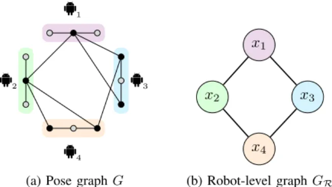
(b) Robot-level graphGR Fig. 1:(a) Example pose graphGwith4robots, each with3poses. Each edge denotes a relative pose measurement (edge direction is omitted). Private poses are colored in gray. (b) Corresponding robot-level graph GR. Two robots are connected if they share any relative measurements (inter-robot loop closures). Note that for robotito optimize its pose estimatesxi, it only needs to receive its neighboring poses through the network. At any time, robotidoes not need to know the private poses of any other robots.

B. Asynchronous Parallel Optimization

The aforementioned works are promising, but critically rely on synchronization that limits their practical value for networked autonomous systems. However, we note that within the broader optimization literature, there is a plethora of works on parallel and asynchronous optimization, partially motivated by popular applications in large-scale machine learning and deep learning. Study of asynchronous gradient-based algorithms began with the seminal work of Bertsekas and Tsitsilis [3], and have led to the recent development of asynchronous randomized block coordinate and stochastic gradient algorithms – see [4]–[7], [19]–[21] and references therein. We are especially interested in asynchronous parallel schemes for non-convex optimization, which have been stud-ied in [7], [21]. In this work, we generalize these approaches to the setting where the feasible set is a the product of non-convex matrix manifolds, motivated by PGO. Our model of asynchrony is comparable to [20]: workers exchange local models asynchronously during optimization. However, unlike [20], we obviate the need for local averaging to achieve consensus, as each robot is only responsible for updating its own trajectory.

III. PROBLEMFORMULATION A. Pose Graph Optimization

In this section, we formally define pose graph optimization (PGO) in the context of multi-robot SLAM. Given relative pose measurements (possibly between different robots), we aim tojointlyestimate the trajectories of all robots in a global reference frame. LetR={1,2, . . . , n}be the set of indices associated withnrobots. Denote the pose of roboti∈ Rat time stepτasTiτ = (Riτ, tiτ)∈SE(d), whered∈ {2,3}is

the dimension of the estimation problem. HereRiτ ∈SO(d)

is a rotation matrix, and tiτ ∈ R

d _{is a translation vector.}

A relative pose measurement fromTiτ toTjs is denoted as

e

Tiτ js = (Re

iτ js,et

iτ

model for our measurements,

e

Riτ js =R

iτ jsR

_{, R∼Langevin(I}

d, wR), (1)

e

tiτ_j s=t

iτ js+t

_{, t∼ N(0, w}−1

t Id). (2)

Above, Tiτ_js = (Riτ_js, tiτ_js) ∈ SE(d) denotes the groundtruth (i.e., noiseless) relative transformation. The isotropic Langevin distribution on rotations [8] plays an analogous role as the multivariate normal distribution on translations. Assuming the relative measurements are free of outliers, the above noise model is thus well-suited and has become the default setup in recent work [2], [8], [9].1

Given noisy observations of the form (1) - (2), we seek to find the maximum likelihood configurations of pose graphs for all robots inR. Doing so amounts to the following non-convex program [8],

Problem 1(Maximum Likelihood Estimation).

min X

(iτ,js)∈E wR

Rjs−RiτRe

iτ js

2

F

+wt

tjs−tiτ −Riτet

iτ js

2 2,

s.t. Riτ ∈SO(d), tiτ ∈R

d_{, ∀i∈ R, ∀τ. (P}

1)

Problem (P1) can be compactly represented with a pose

graph G _, (V, E), where each vertex in V corresponds to a single pose owned by a robot. Observe that the sum in the objective is taken over all edges in E, and directed edges fromiτ tojstoEare formed when there is a relative

measurement fromTiτ toTjs. Figure 1a shows an example

pose graph.

In this paper, we further consider the rank-restricted semidefinite relaxationof (P1) [9]. Define the Stiefel

mani-fold as St(d, r)_,{Y ∈Rr×d :Y>T =Id}, where r≥d

[10]. The rank-rrelaxation of (P1) is defined as the following

non-convex Riemannian optimization problem.

Problem 2(Rank-r-restricted Semidefinite Relaxation).

min X

(iτ,js)∈E wR

Yjs−YiτRe iτ js

2

F

+wt

pjs−piτ −Yiτet

iτ js

2 2,

s.t. Yiτ ∈St(d, r), piτ ∈Rr, ∀i∈ R, ∀τ. (P2)

Observe that forr=d, the Stiefel manifold is identical to the orthogonal group St(d, d) = O(d). In this case, (P2) is

referred to as theorthogonal relaxationof (P1), obtained by

dropping the determinant constraint onSO(d). Asrincreases beyondd, we obtain a hierarchy of rank-restricted problems, each having the form of (P2) but with a slightly “lifted”

search space as determined by r. This hierarchy of rank-restricted problems lies at the heart of the so-called Rieman-nian Staircase procedure [22] for solving the semidefinite relaxation of (P1), which has proven extremely successful in

the design of PGO solvers with global optimality guarantees [2], [8], [9]. Once we solve (P2), either globally or locally

1_{For simplicity, in (1) and (2) we have assumed the same noise parameters}

for all relative measurements. Our approach trivially generalizes to the general case where measurements have distinct measurement noise, as in [2], [8], [9].

to a critical point, we can apply a distributed rounding

procedure (e.g. as detailed in [2]) to obtain an feasible solution to the original MLE problem (P1). Note that (P2)

shares the same sparsity structure as encoded by the pose graph.

For the purpose of designing decentralized algorithms (Section IV), it is more convenient to rewrite (P1) and (P2)

into a more abstract problem one at the level of robots, which may be done as follows.

Problem 3(Robot-level Optimization Problem).

min X

(i,j)∈ER

fij(xi, xj) +

X

i∈R

hi(xi), s.t. xi ∈ Mi, ∀i∈ R.

(P)

In (P), each variable xi concatenates all variables owned

by robot i ∈ R. For instance, for (P2), xi contains all the

“lifted” rotation and translation variables of robot i. Let ni

be the number of poses of roboti. Then, xi=

Yi1 pi1 . . . Yini pini

, (5)

Mi= (St(d, r)×Rr)ni. (6)

The cost function in (P) consists of a set of shared costs fij : Mi× Mj → R between pairs of robots, and a set

of private costs hi : Mi → R for individual robots. For

both (P1) and (P2), fij is formed by relative measurements

between any of robot i’s poses and j’s poses. In contrast, hi is formed by relative measurements within roboti’s own

trajectory.

Similar to the way a pose graph is defined, we can encode the structure of (P) using arobot-level graphGR, (R, ER); see Figure 1b.GR can be viewed as a “reduced”

graph of the pose graph, in which each vertex corresponds to the entire trajectory of a single roboti∈ R. Two robotsi, j are connected inGRif they share any relative measurements (iτ, js)∈E. In this case, we call j aneighboring robot of i, andjsaneighboring poseof robot i.

In the literature, neighboring poses are also referred to as the separators [1]. If a pose variable is not a neighboring pose to any other robots, we call this pose a private pose

[2]. We note that for robotito evaluate the shared costfij,

it only needs to know its neighboring poses in robot j’s trajectory (see Figure 1). This property is crucial to preserve theprivacyof participating robots [1], [2], i.e., at any time, robot does not need to share its private poses with any of its teammates.

IV. PROPOSEDALGORITHM

We present our main algorithm, Asynchronous Stochastic Parallel Pose Graph Optimization (ASAPP), for solving distributed PGO problems of the form (P). Our algorithm is inspired by asynchronous stochastic coordinate descent (e.g., see [6]), in which multiple processors update randomly selected coordinates of the variable concurrently. In the context of distributed PGO, each coordinate corresponds to the stacked relative pose observationsxiof a single robot as

In a practical multi-robot SLAM scenario, each robot can optimize its own pose estimates at any time, and can additionally share its (non-private) poses with others when communication is available. Correspondingly, each robot running ASAPP has two concurrent onboard processes, which we refer to as the optimization thread and com-munication thread. We emphasize that the robots perform both optimization and communication completely in parallel and without synchronization with each other. We begin by describing the communication thread and then proceed to the optimization thread. Without loss of generality, we describe the algorithm from the perspective of roboti∈ R.

A. The Communication Thread

As part of the communication module, each robot i ∈ R implements a local data structure, called a cache, that contains the robot’s own variablexi, together with the most

recent copies of neighboring poses received from the the robot’s neighbors. We note that since onlyi can modifyxi,

the value ofxi in roboti’s cache is guaranteed to be

up-to-date at anytime. In contrast, the copies of neighboring poses from other robots can be out-of-datedue to communication delay. For example, by the time robot i receives and uses a copy of robotj’s poses,j might have already updated its poses due to its local optimization process. In Section V, we show that ASAPP is resilient against such network delay. Nevertheless, for ASAPP to converge, we still assume that the total delay induced by the communication process remainsbounded. We formally introduce this assumption in Section V.

The communication threads performs the following two operations over the cache.

•Receive: After receiving an updated neighboring pose, e.g.,

(Rjs, tjs)from a neighboring robot j over the network, the

communication thread updates the corresponding entry in the cache to store the new value.

• Send: Periodically (when communication is available), robotialso transmits its latest estimatexito its neighboring

robots. Recall from Section III that robotidoes not need to send its private poses, as these pose are not needed by other robots to optimize their estimates.

B. The Optimization Thread

Concurrent to the communication thread, the optimization thread is invoked by a local clock that ticks according to a Poisson process of rateλ >0.

Definition 1 (Poisson process [23]). Consider a sequence

{X1, X2, ...} of positive, independent random variables that

represent the time elapsed between consecutive events (in this case, clock ticks). Let N(t) be the number of events up to timet≥0. The counting process{N(t), t≥0}is a Poisson process with rateλ >0if the interarrival times{X1, X2, ...}

have a common exponential distribution function,

P(Xk≤a) = 1−e−λa, a≥0. (7)

The use of Poisson clocks originates from the design of randomized gossip algorithms by Boyd et al. [24] and is a commonly used tool for analyzing the global behavior of distributed randomized algorithms. We assume that the rate parameterλis equal and shared among robots. In practice, we can adjust λbased on the extent of network delay and the robots’ computational capacity. Using the local clock, the optimization thread performs the following operations in a loop.

•Read: For all neighboring robot j∈N(i), read the values ofxj stored in the local cache. Denote the read values asxˆj.

Recall thatxˆjcan beoutdated, for example if robotihas not

received the latest messages from robotj. In addition, read the value ofxi, denoted asxˆi. Recall from Section IV-A that ˆ

xi is guaranteed to be up-to-date.

In practice,xˆj only contains the set of neighboring poses

from robot j since fij is independent from the rest of j’s

poses (Figure 1). However, for ease of notation and analysis (Section V), we treatxˆj as if it contains the entire set ofj’s

poses.

•Compute: Form the local cost function for roboti, denoted as gi(xi) : Mi → R, by aggregating relevant costs in (P)

that involvexi,

gi(xi) =hi(xi) +

X

j∈N(i)

fij(xi,xˆj). (8)

Compute the Riemannian gradient at robot i’s current esti-matexˆi,

ηi= gradgi(ˆxi)∈TxˆiMi. (9)

• Update: At the next local clock tick, update xi in the

direction of the negative gradient,

xi←Retrxiˆ(−γηi), (10)

whereγ >0 is a constant stepsize. Equation (10) gives the simplest update rule that robots can follow, and forms the basis of our convergence analysis in Section V. To further accelerate convergence in practice, state-of-the-art solvers often implement a heuristic known as preconditioning [2], [8], [9]. We note that ASAPP can be straightforwardly extended to use preconditioning, by using the following alternative update direction,

xi←Retrxˆi(−γPrecongi(ˆxi)[ηi]). (11)

In (11), Precongi(ˆxi) : TˆxiMi → TxˆiMi is a linear,

symmetric, and positive definite mapping on the tangent space that approximates the inverse of Riemannian Hessian. Intuitively, preconditioning helps first-order methods to ben-efit from using the (approximate) second-order geometry of the cost function, which often results in significant speedup especially on poorly conditioned problems.

C. Implementation Details

To make the local clock model valid, we require that the total execution time of theRead-Compute-Updatesequence be smaller than the interarrival time of the Poisson clock,

Algorithm 1 GLOBALVIEW OFASAPP (For Analysis Only)

Input:

Initial solution x0_{∈ Mand stepsize γ >0.}

1: forglobal iteration k= 0,1, . . .do

2: Select robotik ∈ Runiformly at random. 3: Readxˆik=x

k ik. 4: Readxˆjk =x

k−B(jk)

jk , ∀jk ∈N(ik). 5: Compute local gradientηk

ik= gradgik(ˆxik). 6: Updatexk_i+1

k = Retrxˆik(−γη k ik). 7: Carry over allxk_j+1=xk

j, ∀j6=ik. 8: end for

so that the current sequence can finish before the next one starts. This requirement is fairly lax in practice, as all three steps only involve minimal computation and access to local memory. In the worst case, since the interarrival time is determined by 1/λ on average [23], one can also decrease the clock rate λto create more time for each update.

In addition, we note that although the optimization thread and communication thread run concurrently, minimal syn-chronization is required to ensure the so-calledatomic read and write of individual poses. Specifically, a thread cannot read a pose in the cache if the other thread is actively modi-fying its value (otherwise the read value would not be valid). Such synchronization can be easily enforced using software locks. In practice, however, due to the large number of poses owned by each robot, the aforementioned synchronization only happens relatively rarely.

V. CONVERGENCEANALYSIS A. Global View of the Algorithm

In Section IV, we described ASAPP from the local perspective of each robot. For the purpose of establishing convergence, however, we need to analyze the systematic behavior of this algorithm from a global perspective [6], [19], [20], [24]. To do so, letk= 0,1, . . .be a virtual counter that counts the total number ofUpdateoperations applied by all robots. In addition, let the random variableik∈ Rrepresent

the robot that updates at global iteration k. We emphasize thatk andik are purely used for theoretical analysis, and is

in practice unknown to any of the robot.

Recall from Section IV-B that all Update steps are gen-erated by n = |R| independent Poisson processes, each with rate λ. In the global perspective, merging these local processes is equivalent to creating a single, global Poisson clock with rate λn[23]. Crucially, this implies that at any time, all robots have equal probabilities of generating the next Update step, i.e., for all k ∈_N, ik is i.i.d. uniformly

distributed over the set R.

Using this result, we can write the iterations of ASAPP from the global view; see Algorithm 1. We use xk

,

xk

1 xk2 . . . xkn

to represent the value of all robots’ poses after global iterationk. Note thatxlives on the product manifoldM_,M1× M2×. . .Mn. At global iterationk,

a robot ik is selected from Runiformly at random (line 2).

Robotik then follows the steps in Section IV-B to update its

own variable (line 3-6), while all other robots do not update (line 7). Note that in the pseudocode, we have used the fact that ˆxik is always up-to-date (line 3), whilexˆjk is outdated

forB(jk)global iterations (line 4). B. Sufficient Conditions for Convergence

We establish sufficient conditions for ASAPP to converge to first-order critical points.2 _{We adopt the commonly used}

partially asynchronousmodel [3], which assumes that delay caused by asynchrony is not arbitrarily large. In practice, the magnitude of delay is affected by various factors such as the frequency of communication (Section IV-A), the frequency of local optimization (Section IV-B), and intrinsic network latency. For the purpose of analysis, we assume that all these factors can be summarized into a single constant B, which bounds the maximum delay in terms of number of

global iterations(i.e.Update steps applied by all robots) in Algorithm 1.

Assumption 1(Bounded Delay). In Algorithm 1, there exists a constantB >0 such thatB(jk)≤B for all k∈N.

For both the MLE problem (P1) and its rank-restricted

semidefinite relaxations (P2), the gradients of the cost

func-tions enjoy a Lipschitz-type condition, which is proved in our previous work [2] and will be used extensively in the rest of the analysis.

Lemma 1 (Lipschitz-type gradient for pullbacks [2]). De-note the cost function of (P1) and (P2) as f : M → R.

Define the pullback cost as fˆx , f ◦Retrx : TxM →R.

There exists a constantL≥0 such that for anyx∈ Mand η∈TxM,

fˆx(η)−[f(x) +hη,grad_xfi] ≤

L 2 kηk

2

. (12) The condition (12) is first proposed by [25] as an adap-tation of Lipschitz continuous gradient to Riemannian op-timization. Using the bounded delay assumption and the Lipschitz-type condition in (12), we can proceed to analyze the change in cost function after a single iteration of Algo-rithm 1 (in the global view). We formally state the result in the following lemma.

Lemma 2 (Descent Property of Algorithm 1). Under As-sumption 1, each iteration of Algorithm 1 satisfies,

f(xk+1)−f(xk)≤ −γ

2

grad_i

kf(x k₎

2

−γ−Lγ

2

2

η_ik

k

2

+∆BL

2_α2_γ3

2

X

jk∈N(ik) k−1

X

k0_=k−B

η

k0 jk

2

, (13)

where α > 0 is a constant related to the retraction, and ∆>0 is the maximum degree of the robot-level graphGR.

In (13), the last term on the right hand side sums over quantities from earlier iterations, and is a direct consequence of delay in the system. This term is the main obstacle for proving convergence in the asynchronous setting. Indeed, without this term, it is straightforward to verify that any stepsize that satisfies 0 < γ < 1/Lguarantees f(xk+1_{) ≤}

f(xk_{), and thus leads to convergent behavior. With this term,}

however, the overall cost could increase after each iteration. While the delay-dependent error term gives rise to addi-tional challenges, our next theorem states that with suffi-ciently small stepsize, this error term is inconsequential and ASAPP provably converges to first-order critical points.

Theorem 1(Global convergence of ASAPP). Letf?_{be any} global lower bound on the optimum of (P). Defineρ_,∆/n. Letγ >¯ 0 be an upper bound on the stepsize that satisfies,

2ρα2B2L2γ¯2+Lγ¯−1≤0. (14)

In particular, the following choice of ¯γsatisfies (14): ¯

γ=

(√_1+8ρα2B2₋1

4ρα2_B2_L , B >0,

1/L, B = 0.

(15)

Under Assumption 1, if 0 < γ ≤ γ¯, ASAPP converges to a first-order critical point with global sublinear rate. Specifically, afterK total update steps,

min

k∈[K−1]Ei0:K−1

gradf(xk)

2

≤ 2n(f(x

0_)−f?₎

γK .

(16)

Remark 1. To the best of our knowledge, Theorem 1 establishes the first convergence result for asynchronous algorithms when solving anon-convexoptimization problem over the product of matrix manifolds. While the existence of a convergent stepsize γ¯ is of theoretical importance, we further note that its expression expression (15) offers the correct qualitative insights with respect to various problem-specific parameters, which we discuss next.

Relation with maximum delay (B):γ¯increases as maximum delay B decreases. Intuitively, as communication becomes increasingly available, each robot may take larger stepsize without causing divergence. The inverse relationship between

¯

γandBis well known in the asynchronous optimization lit-erature, and is first established by Bertsekas and Tsitsilis [3] in the Euclidean setting.

Relation with problem sparsity (ρ): γ¯ increases as ρ de-creases. Recall thatρ_,∆/nis defined as the ratio between the maximum number of neighbors a robot has and the total number of robots. Thus, ρ is a measure of sparsity of the robot-level graph GR. Intuitively, as GR becomes sparser,

robots can use larger stepsize as their problems become increasing decoupled. Such positive correlation between ¯γ and problem sparsity has been a crucial feature in state-of-the-art asynchronous algorithms; see e.g., [5].

Relation with problem smoothness (L): From (15), it can been seen that ¯γ increases asymptotically with O(1/L).

Moreover, when there is no delay (B = 0), our stepsize matches the well-known constant of 1/L with which syn-chronous gradient descent converges to first-order critical points; see e.g., [25].

VI. EXPERIMENTALRESULTS

We implement ASAPP in C++ and evaluate its per-formance on both simulated and real-world PGO datasets. We use ROPTLIB [26] for manifold related computations, and the Robot Operating System (ROS) [27] for inter-robot communication. The Poisson clock is implemented by halting the optimization thread after each iteration for a random amount of time exponentially distributed with rate λ(default to1000Hz). Since the time taken by each iteration is negligible, we expect that the practical difference between this implementation and the theoretical model in Section IV-B to be insignificant. All robots are simulated as separate ROS nodes running on a desktop computer with an Intel i7 quad-core CPU and16GB memory.

For each PGO problem, we use ASAPP to solve its rank-restricted semidefinite relaxation (P2) with r = 5. During

optimization, we record the evolution of the Riemannian gradient norm gradf(xk)

, which measures convergence

to a first-order critical point. In addition, we also record the optimality gap f(xk_)−f(x?_{), where the globally optimal}

solution x? _{is computed using the centralized Cartan-Sync}

solver [9]. After optimization, we round the solution to

SE(d) and then compute the rotation and translation root mean squared error (RMSE) with respect to the global minimizer.

A. Evaluation in Simulation

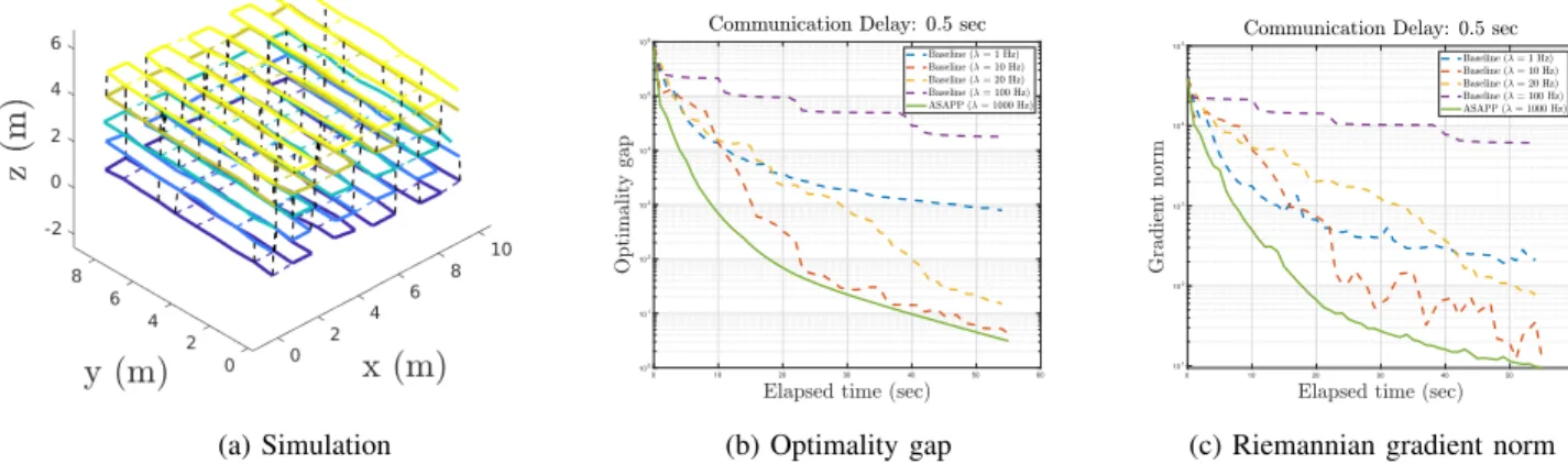
We evaluate ASAPP in a simulated multi-robot SLAM scenario in which5robots move next to each other in a 3D grid with lawn mower trajectories (Figure 2a). Each robot has100poses. With probability0.3, loop closures within and across trajectories are generated for poses within1m of each other. All measurements are corrupted by Langevin rotation noise with standard deviation 2◦, and Gaussian translation noise with standard deviation 0.05 m. To simulate a sce-nario in which robots begin distributed optimization without any prior communication, we initialize each robot’s local trajectory using odometry, while the relative transformations between trajectories are uninitialized. As is commonly done in prior work [4]–[7], [19]–[21], in our experiments we select the stepsize empirically, in this case γ= 5×10−4_.

In the first experiment, we simulate a fixed communication delay by letting each robot communicate every0.5 second. We compare the performance of ASAPP with a baseline algorithm in which each robot uses the second-order Rieman-nian trust-region (RTR) method to optimize its local variable. RTR has emerged as the default solver in the synchronous setting due to its global convergence guarantees and ability to exploit second-order geometry of the cost function. For a comprehensive evaluation, we record the performance of the baseline at different optimization rates (i.e. frequency at which robots update their local trajectories).

(a) Simulation

0 10 20 30 40 50 60

100 101 102 103 104 105 106

(b) Optimality gap

0 10 20 30 40 50 60

101 102 103 104 105

(c) Riemannian gradient norm

Fig. 2: Performance evaluation on 5 robot simulation. The communication delay is fixed at0.5s. We compare ASAPP (with stepsize γ = 5×10−4) with a baseline algorithm in which each robot uses Riemannian trust-region method to optimize its local variables. For a comprehensive evaluation, we run the baseline with varying optimization rate to record its performance under both synchronous and asynchronous regimes. (a) Example trajectories estimated by ASAPP, where trajectories of 5 robots are shown in different colors. Inter-robot measurements (loop closures) are shown as black dashed lines. (b) Optimality gapf(xk_)−f(x?₎

. (c) Riemannian gradient normgradf(xk)

. Note that ASAPP outperforms all variants of the baseline in terms of both optimality gap and gradient norm.

0 5 10 15 20 25 30 35 40 10-2

10-1

100

101

102

103

104

105

Fig. 3:Convergence speed of ASAPP (stepsizeγ= 5×10−4) with varying communication delay. As delay decreases, convergence becomes faster because robots have access to more up-to-date information from each other.

Figure 2b shows the optimality gaps achieved by the evaluated algorithms as a function of wall clock time. The corresponding reduction in Riemannian gradient norm is shown in Figure 2c. Clearly, ASAPP outperforms all variants of the baseline algorithm (dashed curves). We note that the behavior of the baseline algorithm is expected. At a low rate, e.g., λ = 1 Hz (blue dashed curve), the baseline algorithm operates in the synchronous regime and shows convergence behavior. The empirical convergence speed is nevertheless slow, as each robot needs to wait for up-to-date information to arrive after each iteration. At a high rate, e.g., λ= 100Hz (purple dashed curve), robots essentially behave asynchronously. However, since RTR does not regulate the stepsize at each iteration, robots often significantly alter their solutions in the wrong direction (as a result of using outdated information), which again leads to slow convergence or even non-convergence. This comparison demonstrates the advantages offered by ASAPP: while asynchrony effectively reduces the penalty on execution time, the use of conservative stepsize also counters the negative effects of delay and ensures convergence.

In addition, we also evaluate ASAPP under a wide range

of communication delays. Due to space limitation, we only show performance in terms of gradient norm in Figure 3. We note that ASAPP converges in all cases, demonstrating its resilience against various delays in practice. Furthermore, as delay decreases, convergence becomes faster as robots have access to more up-to-date information from each other.

B. Evaluation on benchmark PGO datasets

To further demonstrate the effectiveness of ASAPP, we evaluate the algorithm on several benchmark SLAM datasets. Each dataset is divided into5segments simulating a collabo-rative SLAM mission with5robots.3_{To accelerate empirical}

convergence, we run ASAPP with preconditioning as de-scribed in Section IV-B. To minimize communication usage during initialization, we initialize robots’ trajectory estimates by propagating measurements along a spanning tree of the pose graph. On the syntheticSpheredataset, however, the spanning tree initialization gives a particularly poor initial guess, and we use the distributed chordal initialization [1] instead.

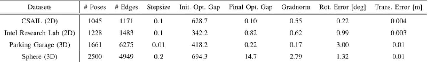
In Table I, we report the performance of ASAPP after running for 60s under a fixed communication delay of 0.1

second. We first note that with preconditioning, ASAPP can afford larger stepsizes (recall that without preconditioning, we need to use a stepsize of 5 × 10−4 _{in the previous}

section). This demonstrates the power of preconditioning in countering the poor conditioning of the optimization problem. Furthermore, on all datasets, ASAPP is convergent and significantly reduces the optimality gap from the initial solution, and the small rotation and translation errors (last two columns) indicate that the solutions are near-optimal.

VII. CONCLUSION

We presented ASAPP, the first parallel and provably delay-tolerant algorithm to solve distributed pose graph optimization and its rank-restricted semidefinite relaxations.

3_{Due to space limitations, figures of these datasets are postponed to the}

TABLE I:Performance of ASAPP with preconditioning on benchmark PGO datasets. Each dataset is divided into trajectories of5robots to simulate a collaborative SLAM scenario. We then run ASAPP for60s under a fixed communication delay of0.1second. For each dataset, we report its size, the stepsize used by ASAPP, and the optimality gaps of the initial and final solution. We also report the final gradient norm achieved with ASAPP, as well as the corresponding rotation and translation root mean squared errors (RMSE).

Datasets # Poses # Edges Stepsize Init. Opt. Gap Final Opt. Gap Gradnorm Rot. Error [deg] Trans. Error [m]

CSAIL (2D) 1045 1171 0.1 628.7 0.10 0.55 0.22 0.004

Intel Research Lab (2D) 1228 1483 0.1 342.2 0.82 0.62 0.99 0.003

Parking Garage (3D) 1661 6275 0.01 418.2 0.22 0.17 3.00 0.01

Sphere (3D) 2500 4949 0.2 694.3 14.7 2.79 1.32 0.01

ASAPP enables each robot to run its local optimization process at a high rate, without waiting for updates from its peers over the network. Assuming a worst-case bound on the communication delay, we established the global first-order convergence of ASAPP, and showed the existence of a convergent stepsize whose value depends on the worst-case delay and inherent problem sparsity. When there is no delay, we further showed that this stepsize matches exactly with the corresponding constant in synchronous algorithms. We performed numerical evaluations on both simulation and real-world datasets, and results confirm the advantages of ASAPP in reducing overall execution time, and demonstrate its resilience against a wide range of communication delay. Our theoretical study in Section V is based on a worst-case analysis and involves unknown constants such as the maximum delay B and Lipschitz constant L. Future work could consider a strategy (e.g., based on average-case analy-sis) that is less conservative and furthermore explicitly deal with the unknown constants in the expression. Another open question is conditions under which stronger performance guarantees may be hold, i.e., local or global extrema. Doing so is challenging due to the geometric aspects of the analysis coming to bear on the non-convexity of the problem, and that typical efforts to improve upon convergence to stationarity require operating inunconstrained settings [28], [29].

REFERENCES

[1] S. Choudhary, L. Carlone, C. Nieto, J. Rogers, H. I. Christensen, and F. Dellaert, “Distributed mapping with privacy and communication constraints: Lightweight algorithms and object-based models,” The International Journal of Robotics Research, vol. 36, no. 12, pp. 1286– 1311, 2017.

[2] Y. Tian, K. Khosoussi, and J. P. How, “Block-coordinate descent on the riemannian staircase for certifiably correct distributed rotation and pose synchronization,” 2019.

[3] D. P. Bertsekas and J. N. Tsitsiklis,Parallel and distributed computa-tion: numerical methods, vol. 23. Prentice hall Englewood Cliffs, NJ, 1989.

[4] A. Agarwal and J. C. Duchi, “Distributed delayed stochastic optimiza-tion,” Advances in Neural Information Processing Systems (NIPS), 2011.

[5] F. Niu, B. Recht, C. Re, and S. Wright, “Hogwild: A lock-free approach to parallelizing stochastic gradient descent,” Advances in Neural Information Processing Systems (NIPS), 2011.

[6] J. Liu and S. J. Wright, “Asynchronous stochastic coordinate descent: Parallelism and convergence properties,”SIAM Journal on Optimiza-tion, 2015.

[7] X. Lian, Y. Huang, Y. Li, and J. Liu, “Asynchronous parallel stochastic gradient for nonconvex optimization,”Advances in Neural Information Processing Systems (NIPS), 2015.

[8] D. M. Rosen, L. Carlone, A. S. Bandeira, and J. J. Leonard, “Se-sync: A certifiably correct algorithm for synchronization over the special euclidean group,” The International Journal of Robotics Research, 2019.

[9] J. Briales and J. Gonzalez-Jimenez, “Cartan-sync: Fast and global se(d)-synchronization,”IEEE Robotics and Automation Letters, Oct 2017.

[10] P.-A. Absil, R. Mahony, and R. Sepulchre,Optimization algorithms on matrix manifolds. Princeton University Press, 2009.

[11] R. Tron and R. Vidal, “Distributed image-based 3-d localization of camera sensor networks,” inProceedings of the 48h IEEE Conference on Decision and Control (CDC) held jointly with 2009 28th Chinese Control Conference, 2009.

[12] R. Tron, Distributed optimization on manifolds for consensus al-gorithms and camera network localization. The Johns Hopkins University, 2012.

[13] R. Tron and R. Vidal, “Distributed 3-d localization of camera sensor networks from 2-d image measurements,” IEEE Transactions on Automatic Control, vol. 59, pp. 3325–3340, Dec 2014.

[14] R. Tron, J. Thomas, G. Loianno, K. Daniilidis, and V. Kumar, “A distributed optimization framework for localization and formation control: Applications to vision-based measurements,” IEEE Control Systems Magazine, vol. 36, pp. 22–44, Aug 2016.

[15] J. Knuth and P. Barooah, “Collaborative 3d localization of robots from relative pose measurements using gradient descent on manifolds,” in 2012 IEEE International Conference on Robotics and Automation, 2012.

[16] S. Choudhary, L. Carlone, H. I. Christensen, and F. Dellaert, “Ex-actly sparse memory efficient slam using the multi-block alternating direction method of multipliers,” in 2015 IEEE/RSJ International Conference on Intelligent Robots and Systems (IROS), 2015. [17] P. Lajoie, B. Ramtoula, Y. Chang, L. Carlone, and G. Beltrame,

“Door-slam: Distributed, online, and outlier resilient slam for robotic teams,” IEEE Robotics and Automation Letters, 2020.

[18] T. Fan and T. D. Murphey, “Generalized proximal methods for pose graph optimization,” in The International Symposium on Robotics Research, 2019.

[19] J. Liu, S. J. Wright, C. R´e, V. Bittorf, and S. Sridhar, “An asynchronous parallel stochastic coordinate descent algorithm,”Journal of Machine Learning Research, 2015.

[20] X. Lian, W. Zhang, C. Zhang, and J. Liu, “Asynchronous decentralized parallel stochastic gradient descent,” in Proceedings of the 35th International Conference on Machine Learning (ICML), 2018. [21] L. Cannelli, F. Facchinei, V. Kungurtsev, and G. Scutari,

“Asyn-chronous parallel algorithms for nonconvex optimization,” Mathemat-ical Programming, 2019.

[22] N. Boumal, “A riemannian low-rank method for optimization over semidefinite matrices with block-diagonal constraints,” 2015. [23] H. Tijms,A First Course in Stochastic Models. John Wiley and Sons,

Ltd, 2004.

[24] S. Boyd, A. Ghosh, B. Prabhakar, and D. Shah, “Randomized gossip algorithms,”IEEE Transactions on Information Theory, vol. 52, no. 6, pp. 2508–2530, 2006.

[25] N. Boumal, P.-A. Absil, and C. Cartis, “Global rates of convergence for nonconvex optimization on manifolds,”IMA Journal of Numerical Analysis, vol. 39, pp. 1–33, 02 2018.

[26] W. Huang, P.-A. Absil, K. A. Gallivan, and P. Hand, “Roptlib: an object-oriented c++ library for optimization on riemannian manifolds,” tech. rep., Florida State University, 2016.

[27] M. Quigley, K. Conley, B. P. Gerkey, J. Faust, T. Foote, J. Leibs, R. Wheeler, and A. Y. Ng, “Ros: an open-source robot operating system,” inICRA Workshop on Open Source Software, 2009. [28] R. Ge, F. Huang, C. Jin, and Y. Yuan, “Escaping from saddle points

– online stochastic gradient for tensor decomposition,” inConference on Learning Theory, pp. 797–842, 2015.

[29] S. Paternain, A. Mokhtari, and A. Ribeiro, “A newton-based method for nonconvex optimization with fast evasion of saddle points,”SIAM Journal on Optimization, vol. 29, no. 1, pp. 343–368, 2019.

APPENDIX A. Proof of Lemma 2

Proof. Suppose that at iterationk, robot ik is selected for update. Recall that xk =

xk

1 xk2 . . . xkn

∈ M, where M is the product manifold M = M1× M2×. . .Mn (Section V-A). For all k ∈ N, define the aggregate tangent vector

ηk_∈T

xkM as,

ηki ,

(

ηk

ik, ifi=ik,

0, otherwise. (17)

By definition ofηk_{, the update step in Algorithm 1 (line 6-7) is equivalent to,}

xk+1= Retrxk(−γηk). (18)

By Lemma 1,f has Lipschitz-type gradient for pullbacks. Therefore, f(xk+1)−f(xk)≤ −γhgradf(xk), ηki+Lγ

2

2

ηk

2

=−γhgrad_i kf(x

k_{), η}k iki+

Lγ2

2

η_ik

k

2

. (19)

Using the equalityhη1, η2i= 1₂[kη1k 2

+kη2k 2

− kη1−η2k 2

], we can convert the inner product that appears on the right hand side of (19) into,

hgrad_ikf(xk), η_ikki=1 2

grad_ikf(xk)

2

+ηk_ik

2

−

grad_ikf(xk)−η_ikk

2

. (20)

Substitute (20) into (19). After collecting relevant terms, we have, f(xk+1)−f(xk)≤ −γhgrad_ikf(xk), ηk_iki+Lγ

2

2

η_ikk

2

=−γ

2

grad_ikf(xk)

2

+η_ikk

2

−

grad_ikf(xk)−η_ikk

2

+Lγ

2

2

ηk_ik

2

=−γ

2

grad_ikf(xk)

2

−γ−Lγ

2

2

η_ikk

2

+γ 2

grad_ikf(xk)−η_ikk

2

.

(21)

We proceed to bound the last term on the right hand side of (21). Recall from (8) and (9) that ηk

ik is formed with stale

gradients,

ηkik = gradikhik(x k ik) +

X

jk∈N(ik)

gradikfek(x k ik, x

k−B(jk)

jk ), (22)

where we abbreviate the notation by definingek,(ik, jk)∈ER. In contrast, the Riemannian gradientgradikf(x k_{)is by}

definition formed using up-to-date variables,

gradikf(x

k_{) = grad} ikhik(x

k ik) +

X

jk∈N(ik)

gradikfek(x k ik, x

k

jk). (23)

Note that the only difference between (22) and (23) is that delayed information is used in (22). In order to form the last term on the right hand side of (21), we subtract (22) from (23) and compute the norm distance. Subsequently, we use the triangle inequality to obtain an upper bound on this norm distance,

grad_i

kf(x k_)−ηk

ik

=

X

ek=(ik,jk)∈ER

grad_i kfek(x

k ik, x

k

jk)−gradikfek(x k ik, x

k−B(jk)

jk )

≤ X

ek=(ik,jk)∈ER

gradikfek(x k ik, x

k

jk)−gradikfek(x k ik, x

k−B(jk) jk )

| {z }

(ik,jk)

.

(24)

Next, we proceed to bound each (ik, jk)term. To do so, we use the fact that for a real-valued function f defined over

a matrix submanifoldM ⊆ E, its Riemannian gradient is obtained as the orthogonal projection of the Euclidean gradient onto the tangent space (see [10, Section. 3.6.1]),

Substituting (25) into the right hand side of (24), it holds that, (ik, jk) =

gradikfek(x k ik, x

k

jk)−gradikfek(x k ik, x

k−B(jk)

jk ) = Proj_T xk ik

∇ikfek(xkik, x k

jk)−ProjTxk ik

∇ikfek(xkik, x k−B(jk)

jk ) . (26)

Furthermore, since the tangent space is identified as a linear subspace of the ambient space E [10, Section 3.5.7], the orthogonal projection operation is a non-expansivemapping, i.e.,

(ik, jk) =

Proj_T xk ik

∇ikfek(xkik, x k

jk)−ProjTxk ik

∇ikfek(xkik, x k−B(jk)

jk ) ≤

∇ikfek(x

k ik, x

k

jk)− ∇ikfek(x k ik, x

k−B(jk)

jk )

.

(27)

Since the norm distance with respect toik is no greater than the overall norm distance, we furthermore have, (ik, jk)≤

∇ikfek(x

k ik, x

k

jk)− ∇ikfek(x k ik, x

k−B(jk)

jk ) ≤ ∇fek(x

k ik, x

k

jk)− ∇fek(x k ik, x

k−B(jk)

jk )

. (28)

In (P), the Euclidean gradient of each cost functionfek is Lipschitz continuous. Furthermore, it is straightforward to show

that the Lipschitz constant offek is always less than or equal to the Lipschitz constant of the overall cost functionf. Denote

the latter asC >0. By definition, we thus have,

(ik, jk)≤C

x

k jk−x

k−B(jk) jk

. (29)

In addition, in [2] we have shown that the Riemannian version of the Lipschitz constant L that appears in Lemma 1 is always greater than or equal to the Euclidean Lipschitz constant C (see Lemma 5 in [2]). Thus,

(ik, jk)≤L

x

k jk−x

k−B(jk) jk

. (30)

We proceed by bounding the norm on the right hand side of (30). Writing the subtraction as a telescoping sum and invoking triangle inequality, we first obtain,

x

k jk−x

k−B(jk) jk =

k−1

X

k0_=k−B(jk)

xk_j0+1 k −x

k0 jk ≤

k−1

X

k0_=k−B(jk)

x

k0+1

jk −x k0 jk

. (31)

Recall that for alljk and iterationsk0, the next iteratexk 0₊₁

jk is obtained fromx k0

jk via the following update, xk_jk0+1= Retr_xk0

jk (−γη_jk0

k). (32)

Furthermore, from Lemma 5 in [2], we know that for each manifoldMi, there exists a corresponding constantαi>0 such

that the Euclidean distance from the initial point to the new point after retraction is always bounded byαi, i.e.,

kRetrx_i(ηi)−xik ≤αikηik, ∀x∈ M, ∀ηi∈TxiM. (33)

Equation (33) thus provides a way to bound the term on the right hand side of (31),

x

k jk−x

k−B(jk)

jk

≤

k−1

X

k0_=k−B(j k)

Retrxk_jk0(−γη

k0 jk)−x

k0 jk

≤

k−1

X

k0_=k−B(j k) αjk γη k0 jk . (34)

To remove the dependency onαjk, letα,maxi∈Rαi. We thus have,

x

k jk−x

k−B(jk) jk

≤αγ

k−1

X

k0_=k−B(jk)

η k0 jk . (35)

We can further more use the bounded delay assumption (Assumption 1) to replaceB(jk)withB,

x

k jk−x

k−B(jk) jk

≤αγ

k−1

X

k0_=k−B(jk)

η k0 jk ≤αγ

k−1

X

k0_=k−B

η k0 jk . (36)

Substituting (36) into (30), we have,

(ik, jk)≤αγL k−1

X

k0_=k−B

η k0 jk . (37)

Substituting (37) into (24), we then have,

grad_i

kf(x k_)−ηk

ik

≤

X

jk∈N(ik)

(ik, jk)≤αγL

X

jk∈N(ik)

k−1

X

k0_=k−B

η k0 jk . (38)

Squaring both sides of (38), we obtain,

grad_i

kf(x k_)−ηk

ik 2 ≤ αγL X

jk∈N(ik)

k−1

X

k0_=k−B

η k0 jk 2

=α2γ2L2

X

jk∈N(ik)

k−1

X

k0_=k−B

η k0 jk 2 . (39)

Recall that the sum of squares inequality states that (Pn

i=1ai)

2 _≤nPn

i=1a 2

i. This gives an upper bound on the squared

term in (39),

grad_i

kf(x k₎

−η_ik k

2

≤α2γ2L2B∆ik

X

jk∈N(ik) k−1

X

k0_=k−B

η k0 jk 2

≤α2γ2L2B∆ X jk∈N(ik)

k−1

X

k0_=k−B

η k0 jk 2 , (40) where∆i_k ≤∆is robotik’s degree in the robot-level graphGR. Finally, substituting (40) in (21) concludes the proof,

f(xk+1)−f(xk)≤ −γ

2

grad_ikf(xk)

2

−γ−Lγ

2

2

η_ikk

2 +γ 2

grad_ikf(xk)−η_ikk

2

(41) ≤ −γ

2

grad_ikf(xk)

2

−γ−Lγ

2

2

η_ik

k

2

+α

2_γ3_L2_B∆

2

X

jk∈N(ik)

k−1

X

k0_=k−B

η k0 jk 2 . (42)

B. Proof of Theorem 1

Proof. Sincef? _{is a global lower bound onf, we can obtain the following inequality,} f?−f(x0)≤Ei0:K−1

f(xK)

−f(x0) =_Ei0:K−1

K−1 X

k=0

(f(xk+1)−f(xk))

, (43)

where the right hand side rewrites the middle term as a telescoping sum. Using the linearity of expectation, we obtain, f?−f(x0)≤Ei0:K−1

K−1 X

k=0

(f(xk+1)−f(xk))

= K−1

X

k=0

Ei0:k

f(xk+1)−f(xk)

. (44)

For each expectation term, applying the law of total expectation yields, f?−f(x0)≤

K−1

X

k=0

Ei0:k−1

Eik|i0:k−1[f(x

k+1_)−f(xk_)]

. (45)

Next, recall that Lemma 2 already gives an upper bound on the innermost term of (45). Substituting this upper bound into (45) gives,

f?−f(x0)≤

K−1

X

k=0

Ei0:k−1

Eik|i0:k−1

−γ

2

gradikf(x k₎

2

−γ−Lγ

2 2 η k ik 2

+∆Bα

2_L2_γ3

2

X

jk∈N(ik) k−1

X

k0_=k−B

η k0 jk 2 . (46) Next, we simplify individual terms on the right hand side of (46). We start with the first conditional expectation term. Using the definition of conditional expectation,

Eik|i0:k−1

−γ

2

grad_ikf(xk)

2

=−γ

2 n

X

i=1

P(ik=i|i0:k−1)

grad_if(xk)

2

. (47)

Recall that{ik}are i.i.d. random variables uniformly distributed over1ton(Section V-A). SettingP(ik=i|i0:k−1) = 1/n

thus gives,

Eik|i0:k−1

−γ

2

grad_ikf(xk)

2

=−γ

2 n X i=1 1 n

grad_if(xk)

2

=− γ

2n

gradf(xk)

2

. (48)

Similarly, for the third conditional expectation in (46), we note that,

Eik|i0:k−1

X

jk∈N(ik) k−1

X

k0_=k−B

η k0 jk 2 = n X i=1 1 n X

j∈N(i)

k−1

X

k0_=k−B

η k0 j 2 . (49)

In equation (49), exchange the order of summations and collect relevant terms, n X i=1 1 n X

j∈N(i)

k−1

X

k0_=k−B

η k0 j 2 = 1 n

k−1

X

k0_=k−B n

X

i=1

X

j∈N(i)

η k0 j 2 = 2 n

k−1

X

k0_=k−B

η k0 2 . (50)

Using our simplified expressions for the first and third term on the right hand side of (46), we obtain, f?−f(x0)≤

K−1

X

k=0

Ei0:k−1

− γ

2n

gradf(xk)

2

−_Eik|i0:k−1

_γ−Lγ2

2

η_ik

k

2

+∆Bα

2_L2_γ3

n

k−1

X

k0_=k−B

η k0 2 . (51) Next, using the independence relations and the linearity of expectation, we obtain,

f?−f(x0)≤Ei0:K−1

K−1

X k=0 − γ 2n

gradf(x

k )

2

−γ−Lγ

2 2 η k 2

+∆Bα

2_L2_γ3

n

k−1

X

k0_=k−B

η k0 2 . (52) At this point, our bound still involves the squared norms of update vectors from earlier iterations (last term on the right hand side). To simplify the bound further, note that,

K−1

X

k=0

k−1

X

k0_=k−B

η k0 2 ≤B K−1

X k=0 ηk 2 . (53)

Using the above inequality in (52), we obtain, f?−f(x0)≤_Ei0:K−1

K−1

X k=0 − γ 2n

gradf(xk)

2

+ (∆α

2_B2_L2_γ3

n +

Lγ2_−γ

2 )

| {z }

A1(γ)

ηk 2 . (54)

We establish a sufficient condition on γ such that A1(γ) as a whole is nonpositive. Let us define ρ,∆/n. Consider the

following factorization ofA1(γ),

A1(γ) =

γ 2 (2ρα

2_B2_L2_γ2_+Lγ−1)

| {z }

A2(γ)

. (55)

Note thatA2(γ)is the same as (14) in Theorem 1. For the moment, suppose that we can findγ >0 such thatA2(γ)≤0.

This implies that A1(γ)≤0, and we can thus drop this term on the right hand side of (54),

f?−f(x0)≤≤ − γ

2n K−1

X

k=0

Ei0:K−1

gradf(xk)

2

. (56)

Replacing the expected value at each iteration with the minimum across all iterations, we have, f?−f(x0)≤ −γK

2n k∈min[K−1]Ei0:K−1

gradf(xk)

2

. (57)

Finally, rearranging the last inequality yields,

min

k∈[K−1]Ei0:K−1

gradf(xk)

2

≤2n(f(x

0_)−f?₎

γK . (58)

Thus we have proved the main part of Theorem 1. To prove the expression (15), note that ifB = 0(i.e., there is no delay), the condition A2(γ)≤0 entails Lγ ≤1. In this case, we can thus set the upper bound γ¯ to1/L. On the other hand, if

B >0,A2(γ)becomes a quadratic function ofγ, and furthermore has the following positive root,

¯ γ=

p

1 + 8ρα2_B2₋₁

4ρα2_B2_L >0. (59)

It is straightforward to verify that A2(γ)≤0for allγ∈(0,¯γ]. Therefore, we have proved that the conditionA2(γ)≤0 is

ensured by the following choice ofγ¯,

¯ γ=

(√_1+8ρα2B2₋1

4ρα2_B2_L , B >0,

1/L, B= 0.

(60) In particular, under this choice, ASAPP converges globally to first-order critical points, with an associated convergence rate given in (58).

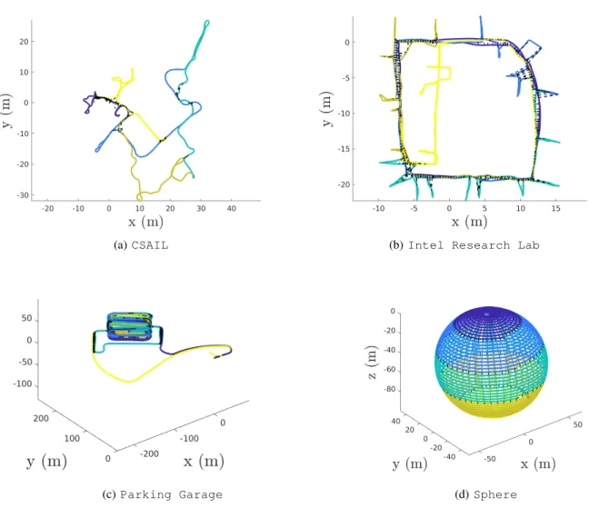
(a)CSAIL (b)Intel Research Lab

(c)Parking Garage (d)Sphere

Fig. 4:Trajectory estimates returned by ASAPP on benchmark datasets. Each dataset contains trajectories of 5 robots (different colors). Inter-robot measurements (loop closures) are shown as black dashed lines. (a) CSAIL; (b)Intel Research Lab; (c) Parking garage; (d)Sphere.