Oil Price Elasticities and Oil Price Fluctuations

(1)

Oil Price Elasticities and Oil Price Fluctuations

∗

Dario Caldara

†

Michele Cavallo

‡

Matteo Iacoviello

§

April 18, 2016

Abstract

We study the identification of oil shocks in a structural vector autoregressive (SVAR) model of the oil market. First, we show that the cross-equation restrictions of a SVAR impose a nonlinear relation between the short-run price elasticities of oil supply and oil demand. This relation implies that seemingly plausible restrictions on oil supply elasticity map into implausible values of the oil demand elasticity, and vice versa. Second, we propose an identification scheme that restricts the values of these elasticities by minimizing the distance between the SVAR-implied elasticities and target values that we construct by surveying the relevant studies. Third, we use the identified SVAR to analyze sources and consequences of movements in oil prices. We find that (1) oil supply shocks and global demand shocks explain 50 percent and 30 percent of oil price fluctuations, respectively; (2) a drop in oil prices driven by supply shocks boosts economic activity in advanced economies, whereas it depresses economic activity in emerging economies, thus helping explain the muted effects of changes in oil prices on global economic activity; and (3) the selection of oil market elasticities is essential to understanding the nature of oil price movements and to measuring the size of the multipliers of oil prices on economic activity.

∗_{J Seymour and Lucas Husted provided outstanding research assistance. The views expressed in this paper are solely}

the responsibility of the authors and should not be interpreted as reflecting the views of the Board of Governors of the Federal Reserve System or of anyone else associated with the Federal Reserve System.

†

Federal Reserve Board. E-mail: dario.caldara@frb.gov

‡

Federal Reserve Board. E-mail: michele.cavallo@frb.gov §

(2)

1 Introduction

Major swings in the price of oil—such as the ongoing persistent slump that started in 2014—draw a lot of attention among policymakers, academics, and practitioners. A common theme in the academic literature, as well as in the economic and financial press, is that these swings reflect a variety of structural forces. On the demand side, as crude oil is one of the most important source of energy worldwide, oil prices are considered to be an important indicator of the strength of global demand, with oil price movements thus believed to reflect the variability of the global business cycle. On the supply side, oil production is concentrated in a few, and mostly politically unstable, regions, making the oil market particularly susceptible to supply disruptions. As a byproduct of the potentially unstable supply, and because crude oil is a widely traded commodity, oil prices are also driven by precautionary demand and by speculation in futures markets.

Understanding what causes movements in oil prices is important for forecasting and for assessing the consequences for the global economy. Empirically distinguishing among competing sources of fluc-tuations, however, has proved to be a particularly difficult task. To achieve this goal, we study the identification of oil shocks in a structural vector autoregressive (SVAR) model of the oil market using a new methodology and new data. Using the identified shocks, we provide a full characterization of the two-way interaction between the oil market and the global economy, with a particular focus on the determinants of oil prices and on the differential effect of oil shocks on advanced and emerging economies.

Our methodological contribution aims at distinguishing supply and demand shocks in driving oil prices and oil production. Doing so requires identifying supply and demand shocks. A stark illustration of this identification problem is depicted in figure 1, which shows the scatter plot between monthly surprises in oil prices and oil production implied by simple univariate AR(1) regressions. The dots clearly show that oil prices and oil production are uncorrelated.1

The lack of correlation between prices and production could be the outcome of very different oil market configurations and, by implication, could be explained by very different combinations of supply and demand shocks. For instance, as depicted by the black dashed lines, the supply curve could be inelastic while the demand curve could be very elastic. As a result, fluctuations in oil prices and oil production would be decoupled, with prices driven uniquely by demand shocks and production driven uniquely by supply shocks. A market characterized by a very elastic oil supply curve and a very inelastic demand curve, as in the blue dotted lines, would also lead to a decoupling of movements in oil prices and oil production. In between, as depicted by the red solid lines, lies an oil market with a downward-sloping demand curve and an upward-sloping supply curve, which would imply that demand and supply shocks

(3)

jointly affect oil prices and production. Those market configurations, which we picked among many for illustrative purposes, are equally consistent with the data but, as we will show, have very different implications not only for the causes, but also for the consequences of oil prices fluctuations.

More generally, we formally show that the cross-equation restrictions embedded in SVARs impose a nonlinear relation between the short-run price elasticities of oil supply and oil demand—that is, on the slopes of the curves depicted in figure1. This relation implies that seemingly plausible restrictions on the oil supply elasticity map into implausible values of the oil demand elasticity, and vice versa. We build on this finding and propose an identification scheme that jointly restricts the slope of both the supply and demand schedules by minimizing the distance between the SVAR-implied elasticities and the target values that we recovered through a meta-analysis of relevant studies. These targets are consistent with the conventional view that the short-run price elasticities of both oil supply and demand are small. More precisely, our identification targets a supply elasticity of about 0.10 and a demand elasticity of about −0.10.

Even with this identification strategy at hand, an additional empirical challenge is to disentangle demand shocks that are specific to the oil market from shocks to the demand for oil originating from changes in global economic activity. The main difficulty is that global demand for oil is hard to measure, and, for this purpose, many indicators have been used in the literature. Our approach is to use three indicators of real economic activity to provide a rich and more varied characterization of oil demand. We construct two separate indicators of aggregate activity dating back to the 1980s, one based on industrial production in emerging economies and one based on industrial production in advanced economies. Our third indicator of global activity is an index of industrial metal prices. Metal prices are often viewed by policymakers and practitioners as early indicators of swings in economic activity and global risk sentiment.2

We begin our analysis with a simple forecasting exercise in which we compare the ability of these global activity indicators to predict oil prices. Although industrial production (IP) in emerging economies and the metal price index help predict fluctuations in future oil prices, industrial production in advanced economies does not provide any marginal improvement in forecasting power. Hence, the main reason to include advanced economies’ activity in the SVAR model is to study how oil market shocks influence activity in advanced economies and, by implication, whether the lack of predictive power is due to an endogeneity bias.

We then turn to the analysis of the causes and consequences of oil price movements. Our main findings can be summarized as follows. First, we find that oil price fluctuations are primarily driven by oil market-specific shocks, with oil supply shocks explaining about 50 percent of the volatility in

(4)

oil prices. Second, we find that shocks to global demand explain, on average, about 30 percent of the volatility of oil prices at a two-year horizon. Compared with the forecast regressions, we find that activity in advanced economies has a significant but economically modest effect on oil prices. Moreover, our characterization of global demand is particularly important to understanding the nature of some historical episodes associated with large swings in oil prices, such as the Asian financial crisis and the recent slump in oil prices that started in June 2014. Third, we find that a drop in oil prices driven by oil market shocks, regardless of whether the shock originates from supply or demand, depresses economic activity in emerging economies. Fourth, a drop in oil prices boosts economic activity in advanced economies only if it is supply driven. Given the historical realization of these oil shocks, these findings help rationalize the muted effects of changes in oil prices on global economic activity.

Our paper contributes to the expanding literature that uses SVARs to study the interaction between the oil market and macroeconomic variables. Since Kilian (2009), several studies have emphasized the importance of imposing plausible restrictions on the oil supply elasticity.3 Unlike these papers, we jointly select oil supply and demand elasticities in a way that is coherent with both external information and the observed equilibrium relationships in the data. Our approach is also related to the recent study of Baumeister and Hamilton (2015b), who impose plausible prior distributions on both the oil supply and demand elasticities to identify oil shocks.4 _{Compared with that study, we show that (i) the} decomposition of movements in oil prices is extremely sensitive to the assumptions on both the supply and demand elasticities and (ii) small differences in the values of the elasticities have a substantial effect on inference. We also show that, in the language ofBaumeister and Hamilton(2015b), one could discipline the identification of the SVAR by imposing joint, rather than independent, prior distributions on oil market elasticities.

Regarding the data, our analysis builds on the seminal paper by Kilian (2009), who constructs a new monthly measure of global real economic activity based on data for dry cargo bulk freight rates. As explained earlier, we replace his measure with three indicators to provide a richer characterization of the global demand for oil. The use of IP follows recent work byAastveit et al. (2015), who analyze the contribution of demand from advanced and emerging economies to movements in the real price of oil using a factor-augmented vector autoregressive (FAVAR) model. The use of metal prices as an indicator of real activity has also been proposed byArezki and Blanchard(2014), whose analysis exploits the idea that metal prices typically react to global activity even more than oil prices.5 _Similarly,_Bernanke₍₂₀₁₆₎ argues that prices of commodities such as copper can act as indicators of underlying global growth, as

3_{See, for instance,}_{Kilian and Murphy}₍₂₀₁₂_{) and}_{Kilian and Murphy}₍₂₀₁₄_). 4_{See also}_{Baumeister and Hamilton}₍_2015a_).

5_Hamilton₍₂₀₁₄_{) has, around the same time, put forward the notion that concurrent swings in the prices for oil and} metals could be indicative of changes in global demand.

(5)

they are likely to respond to investors’ perceptions of global demand and not so much to changes in oil supply.6

The inclusion of a broader set of indicators of global demand boosts the estimated contribution of global business cycle fluctuations to oil price movements. For instance, our identified global demand shocks explain about 25 percent of the historical fluctuations in oil prices, compared with the 8 percent estimate obtained using the preferred model in Kilian(2009) and the 4 percent estimated contribution documented in Baumeister and Hamilton (2015b). Nonetheless, the contribution of global demand shocks is smaller than the 50 percent estimate reported inAastveit et al. (2015), with the key difference being the larger contribution of the global demand for oil in advanced economies compared with our estimates.

The paper is structured as follows. Section 2 describes the indicators of global activity and their ability to capture the demand for oil. Section 3 discusses the econometric framework and the identifi-cation strategy. Sections4 presents the main results. Section 5investigates the importance of selecting plausible oil elasticities. Section 6concludes.

2 Measuring Global Demand for Oil

2.1 Overview

An empirically compelling structural model of the oil market must be able to separate the responses of oil market variables to oil-specific shocks from those to global economic developments. With this goal in mind, we select global economic indicators that fulfill two requirements: First, they must capture key salient features of the global business cycle, and, second, they must be good predictors of the global demand for oil. Rather than taking a stand on one single measure, we consider four different monthly indicators. In this section we describe the indicators, their properties, and their roles as predictors of global oil demand.

2.2 Indicators of Global Activity

Our first two indicators of global activity are based on cross-country data on IP. We use data on IP for three reasons: (1) IP is widely available across a large number of economies, advanced and emerging

6_{Market analysts as well as the economic and financial press recently hinted that aluminum can also play the role of} thermometer of global demand conditions, especially at a time when copper prices are declining while the global economy continues to grow. Aluminum is used in a vast range of products and its market size is twice the size of the copper market. See “Is Aluminum the New Doctor Copper?” by Ese Erheriene,Wall Street Journal, Jan 29, 2015, available at

(6)

alike; (2) IP is historically a very reliable business cycle indicator;7 _{and (3) IP can capture the demand} for oil better than other indicators of real activity covering government and service sectors, as oil is an important factor of production in the industrial sector. To measure IP on a global scale, we construct two indexes that aggregate IP data for advanced economies (ya) and for emerging economies (ye).

The split between advanced and emerging economies is dictated by two pieces of evidence, which are summarized in detail in Appendix A.8 _{First, emerging economies use relatively more oil than advanced} economies. In particular, even if emerging economies produce a much smaller share of global GDP than advanced economies, their share of global oil consumption is similar. As a consequence, the effect on oil demand of a given change in IP from either group could be different. Second, emerging economies are—as a whole—oil independent, while advanced economies are—as a whole—net oil importers. In particular, emerging economies in our sample produce about 35 percent and absorb about 40 percent of global oil availability. By contrast, the advanced economies produce 20 percent and consume 40 percent of global oil availability. As a consequence, the effect on IP in advanced and emerging economies of a given oil shock could be different too.

Although intuitive and readily available, IP may be a lagging indicator of global oil demand, as it may take time to alter production schedules in reaction to changing market conditions because of the presence of various types of adjustment costs. For this reason, we also consider two potential leading indicators of the global business cycle. The first indicator is the International Monetary Fund (IMF) metal price index (m). Base metals are the lifeblood of industrial activity, as they are critical material inputs in sectors whose cycles are normally synchronized such as capital equipment and heavy manufacturing, construction, infrastructure investment, and consumer durables. Moreover, production plans in these sectors are typically set up in advance, and, thus, purchase decisions for metal inputs are necessarily based on expectations of future market conditions. As a consequence, metal prices represent an ideal bellwether of shifts in current and expected economic activity at the global level.9

There is an extensive body of literature that supports our choice to include metal prices as indicators of the health of the global economy. The notion that movements in a set of commodity prices may be informative about expectations of global demand and macroeconomic conditions in general was originally investigated byPindyck and Rotemberg(1990), who found that that co-movements in commodity prices can be indicative of shifts in market participants’ expectations about the future paths of macroeconomic

7_{See, for instance,}_{http://www.nber.org/cycles/dec2008.html}_.

8_Appendix _A _{describes in the detail the construction of the IP indexes. Because of the availability of monthly IP} data, our sample includes economies that account for 90 percent of global GDP (excluding both advanced and emerging economies somewhat proportionally), 55 percent of global oil production (because many oil producers do not have reliable IP data), and 80 percent of global oil consumption.

9_IMF₍_2015a_{) provide an in-depth analysis of metal markets in the global economy. See also} _{Arezki and Matsumoto} (2014).

(7)

variables. Similarly, using factor analysis, Labys et al. (1999) show that movements in the common metal price factor appear to be led by fluctuations in the overall OECD industrial production index.10 In more recent related work, Lombardi et al. (2012) document that global economic activity responds positively to higher metal prices as captured by shocks to the common metal factor, thus lending empirical credibility to the idea that co-movements in metal prices reflect anticipations about the pace of expansion in global economic activity.11

The second indicator is the index of global real economic activity (rea) proposed by Kilian (2009) based on dry cargo ocean freight rates. This index is designed to capture shifts in the demand for industrial commodities and, similarly to the metal price index, should capture expected changes in global activity. All series are made stationary by removing a linear trend.

Table 1shows the contemporaneous correlations among these variables over the 1985:M1–2015:M12 period corresponding to the sample used in the vector autoregressive (VAR) analysis that follows. We set 1985 as the starting date because of incomplete data availability for emerging economies IP prior to this date.12

The IP indexes of advanced and emerging economies are negatively correlated. Metal prices display a highly positive correlation with emerging economies’ IP but are negatively correlated with advanced economies’ IP. Finally, rea co-moves with all other indicators, in line with the interpretation in Kilian

(2009) that it represents a broad indicator of global activity. All told, the different correlations suggest that these indicators may capture distinct aspects of the global business cycle.

Do metal prices and the global real activity index lead the business cycle? To test this hypothesis, we look at the ability of m and reato predict activity in advanced and emerging economies by estimating the following forecasting regression:

yt+h =α+β1mt+β2reat+ 12 X i=1 ρ_iyt−i+ 12 X i=1 δ1,imt−i+ 12 X i=1 δ2,ireat−i+t+h, (1)

whereh ≥0 is the forecast horizon,yt={yat, yet},t+h is the forecast error, andρandδare coefficients

that control for past observations. Our interest is in understanding the different predictive power of m andreafor eitheryaorye, as measured byβ₁ andβ₂,once the past state of the economy is conditioned

10_{Barsky and Kilian} ₍₂₀₀₁_{) also draw attention to the striking empirical regularity by which, since the early 1970s,} episodes of sustained increases in non-oil industrial commodity prices were consistent with a picture of rising global demand for all commodities, as those increases were too broad based to reflect commodity-specific supply shocks in individual markets.

11_{Other studies that find a meaningful link between cyclical fluctuations in global economic activity and movements in} metal prices includeCuddington and Jerrett(2011),Issler et al.(2014),Delle Chiaie et al.(2015), andStuermer(2016). 12_{Although IP data are available for a handful of emerging economies starting in the 1960s, 1985:M1 is the earliest} observation when our sample includes enough emerging economies to account, using today’s GDP weights, for at least 25 percent of emerging economies’ aggregate GDP.

(8)

for.

To facilitate the comparison between metal prices and the real economic activity index, we report in table2 the standardized estimates of the coefficientsβ₁ and β₂. Bothm and reahave predictive power for advanced economies’ IP, as shown by panel A. In particular,mpredictsyafor up to a year, whilerea is informative for up to six months and has a lower predictive power thanm. Both indicators are also reliable predictors of near-term economic developments in emerging economies (panel B). At horizons up to one year, the coefficients imply an economically and statistically significant relationship between m, rea, and industrial production, particularly for m. For example, using the standardized estimate ofβ₁ '1 from the regression, an increase of about 30 percent in metal prices in montht—corresponding to a one standard-deviation increase—implies a nearly 4 percent increase in ye—corresponding to a one-standard deviation increase—over a period ranging from six months to about two years. Similarly, using the standardized estimate of β₂ ' 0.2 (an average across the 6, 12 and 24–month horizons), a one standard-deviation increase in rea predicts a 0.8 percent increase in ye six months ahead. In sum, bothm and rea appear to be powerful predictors of economic activity, with the predictive power of m looking more stable across horizons and quantitatively larger. The finding that the predictive power of rea for ya and ye is less stable and quantitatively smaller than that of m is in line with the evidence presented in Beidas-Strom and Pescatori (2014) that swings in rea and in global IP do not always coincide, particularly at times of structural change in the shipping sector.13

2.3 Global Activity as a Predictor of Oil Prices

We now assess the role of the various activity indicators—both the contemporaneous ones, that is, ya and ye, and the “leading” ones, that is,m and rea —in predicting oil prices. Table 3displays pairwise correlations between oil prices (p) and the activity indicators at various leads and lags. The cross-correlation betweenpandyais negative and becomes larger at longer horizons, with oil prices negatively leading ya. The correlations between p and ye and between p and m are positive and large, while the correlations betweenp and rea are positive but small.

To better gauge whether our indexes of global activity capture global demand for oil, we explore

13_{The economic and financial press has also emphasized how the surge in ship delivery and the resulting glut of} large vessels has led to a plunge in dry bulk cargo shipping rates that has hampered the ability of indexes based on those rates to represent a valid gauge of global trade and global economic activity more in general. See, for example, the Financial Timesarticles by Robert Wright, “Dry bulk rates tumble on ship delivery surge,” January 11, 2012, available at

http://www.ft.com/intl/cms/s/0/3db4545a-3c63-11e1-8d38-00144feabdc0.html, and “Shipping costs fall to 25-year low,” February 1, 2012, available athttp://www.ft.com/intl/cms/s/0/743a8bd2-4ce1-11e1-8741-00144feabdc0.html.

(9)

their relative roles in predicting oil prices. Specifically, we estimate the following forecasting regression: pt+h =α+β1yat+β2yet+β3mt+β4reat+ (2) + 12 X i=1 ρ_ipt−i+ 12 X i=1 γ₁_,iyat−i+γ2,iyet−i+γ3,imt−i+γ4,ireat−i +t+h,

whereh≥0 is the forecast horizon,t+his the forecast error, and theρandγare coefficients that control

for past observations. As in the previous set of forecasting regressions, our interest is in understanding the different predictive power of the various economic indicators for oil prices, as measured by the standardized estimates of the coefficients β₁, β₂, β₃, and β₄ (once the past state of the economy is conditioned for).

The results are reported in table 4. Reading across rows shows how the indicators differ sharply in their predictive abilities. The coefficients on ya are not statistically significant, and have the “wrong” sign in that higher IP in advanced economies predicts lower oil prices over a 2-year horizon. Instead, the coefficients on ye and m are positive, and, in general, statistically significant. In particular, the coefficients on m indicate that metal prices are the only indicator with predictive power that extends beyond one year. The coefficients onrea are economically small and not statistically significant.14

Taken together, results from the forecasting exercises show that the marginal contribution ofrea to IP, on the one hand, and to oil prices dynamics on the other, is small once we condition on the other activity indicators in the regressions. For this reason, we leave reaout of the baseline VAR model that follows.15 _{The evidence on the predictive ability of various measures of global activity for oil prices is} mixed, thus suggesting the opportunity to include a broader set of indicators in the VAR model rather than a single one. In particular, the index of metal prices is included in the set of endogenous variables in the VAR also for the purpose of controlling for information that economic agents may have about future global demand and that is not adequately captured by the other activity variables in the system. Of course, the forecasting regressions offer little guidance about the causal relationship between global activity and oil prices. For instance, they are silent on the relative importance of shocks to global activity and shocks to the oil market in shaping the dynamic correlations between these oil and non-oil variables. To address this question empirically, we move to the SVAR analysis, the subject of the remainder of the paper.

14_{Our finding that metal prices have predictive power for oil prices is also consistent with the evidence in}_{Barsky and}

Kilian (2001) that, over the 1975–1985 period, sustained increases in non-oil industrial commodities tended to precede increases in oil prices.

(10)

3 Identifying Oil Market and Global Activity Shocks

3.1 Overview

Suppose that the economic structure describing the oil market and its relationship with the global economy is given by the following SVAR model:

AXt= p X

j=1

αjXt−j +ut, (3)

whereX is a vector of oil market and macroeconomic variables,ut is the vector of structural shocks,p

is the lag length, and A and αj for j = 1, ..., p are matrices of structural parameters. The vector ut is

Gaussian with mean zero and variance-covariance matrixE[utu0t] =Σu. Without loss of generality, we

normalize the entries on the main diagonal of Ato 1 and we assume that Σu is a diagonal matrix. The

reduced-form representation forXt is the following:

Xt = p X

j=1

γ_jXt−j +εt (4)

where the reduced-form residuals εt are related to the structural shocks ut as follows:

εt = But, (5)

Σε = BΣuB0, (6)

where B=A−1, so that, alternatively, ut = Aεt. Estimation of the reduced-form VAR allows to

obtain a consistent estimate of the n(n+ 1)/2 distinct entries of E[εtε0t] = Σε. Hence, to recover the

n2 unknown entries of B and Σu, we need to make (n−1)n/2 identifying assumptions.

To discuss our identification strategy, it is useful to list the set of endogenous variables that we include in the model. The benchmark monthly VAR specification consists of five endogenous variables ordered as follows: (1) log global crude oil production,qt; (2) the log of advanced economies industrial

production,yat; (3) the log of emerging economies industrial production,yet; (4) the log of oil prices,pt;

and (5) the log of the IMF metal price index, mt.

3.2 Identification

We divide the discussion of the identification problem in two steps. First, we discuss the structure we impose on the oil market. Second, we discuss the interaction between the oil market and global activity.

(11)

3.2.1 The Oil Market

Our structural VAR model specifies an oil supply and an oil demand equation, and we interpret inno-vations to these equations as oil supply and oil demand shocks, respectively. After controlling for their own lags and for other determinants of oil supply and demand, these equations define a short-run oil supply curve and a short-run oil demand curve. If we consider a simple bivariate system of order zero inq and p, these curves are defined as follows:

qt = ηSpt+us,t, (7)

qt = ηDpt+ud,t, (8)

where η_S and η_D are the short-run price elasticity of oil supply and oil demand, and us,t and ud,t are

the oil supply and oil demand shocks, assumed to be orthogonal, with standard deviations given byσS

and σD.

The identification problem can be summarized as follows. By construction, the identification of the SVAR has to select parameters that match the estimated variance-covariance matrix of the reduced-form VAR residuals Σε. In the data, the volatility of oil prices is relatively large, the volatility of oil

production is relatively small, and their covariance is close to zero. These three target values can be hit with four structural parameters: the standard deviations of the oil supply and demand shocks as well as the oil supply and demand elasticities. In what follows, we explore how assumptions on the oil demand elasticity restrict the oil supply elasticity, and vice versa. As routine in the literature, we do not directly impose restrictions on the variance of the structural shocks, which are instead pinned down by the restrictions imposed on the elasticities.

Figure2 presents six combinations of slopes of supply and demand schedules in the oil market that could be used to match the data. Panels A and B plot two combinations that achieve the targets. Panel A shows that, given oil supply and oil demand curves, the right mix of supply and demand shocks can generate the “right” volatility of prices and quantities and zero correlation between them. Panel B illustrates another observationally equivalent solution: a highly inelastic supply curve and a highly elastic demand curve. In this case, large demand shocks move oil prices but have negligible effects on oil production, and large supply shocks move oil production but have negligible effects on oil prices. Although the oil market configurations plotted in panels A and B are observationally equivalent, their economic implications are different. When both curves are elastic, oil supply shocks generate a negative co-movement between prices and quantities, while oil demand shocks generate a positive co-movement between prices and quantities. That is, the unconditional zero correlation between prices and quantities observed in the data is accounted by two shocks that generate non-zero conditional correlations. By

(12)

contrast, when the supply curve is inelastic and the oil demand curve is very elastic, there is a disconnect between movements in quantities and movements in prices in the oil market, not only unconditionally, but also conditional on each separate shock.

The remaining panels show why other combinations of supply and demand elasticities are inadmissi-ble. The middle panels (C and D) show that the estimated variance-covariance matrixΣε rules out the

possibility of both highly inelastic supply and inelastic demand. When both the supply and demand curves are inelastic, two configurations may arise. With supply and demand shocks that are both small, the SVAR matches the volatility of prices but underestimates the volatility of oil production (panel C). Alternatively, when both shocks are large, the SVAR can match the volatility of production but overpredicts the volatility of oil prices (panel D).

The lower panels (E and F) illustrate why the estimated variance-covariance matrix Σε also rules

out both highly elastic supply and highly elastic demand. Two configurations may also arise in this case. With supply and demand shocks that are large, the SVAR can match the volatility of prices but overpredicts the volatility of oil production (panel E). Alternatively, with supply and demand shocks that are small, the SVAR can match the volatility of production but underestimates the volatility of oil prices (panel F).16

More formally, given values for the entries of Σε, the variance-covariance structure of the VAR

im-poses a unique relationship between η_S and η_D. The red solid line in figure 3 plots this relationship in our model computed by setting Σε at its OLS estimate.17 The two observationally equivalent

con-figurations depicted in panels A and B of figure 2 denote just two points along a continuum of models that are graphically represented by the curve plotted in figure 3. Along this curve, the likelihood of the VAR is constant, hence there is no statistical basis for preferring one point over another. To choose the “right” elasticities, we need to rely on extra model information.

Our identification proceeds in two steps. First, we search the related empirical literature on oil market price elasticities and compile a list of studies that estimate short-run supply and demand elasticities. We list these studies and the associated elasticities in tableA.4. Only six studies estimate the short-run price elasticity of oil supply: Half of them estimate a supply elasticity of about 0.25, two of them found elasticities near zero, and one study estimates a negative supply elasticity. By contrast, we found thirty studies that estimate the short-run price elasticity of demand. Estimates of the demand elasticity range

16_{One can always find a solution where both supply and demand elasticity have the “right” sign, and the estimated} variances of supply and demand shocks match any desired correlation between prices and production. There are, however, cases in which the solution can call for (1) an upward-sloping demand curve if the correlation between prices and production is large and positive and the supply elasticity is assumed to be “large” or (2) a downward-sloping supply curve if the correlation between prices and production is large and negative and the demand elasticity is assumed to be “large” in absolute value.

17_{We extract the entries of}_Σε _{related to oil prices and quantities from the five-equation VAR. The estimation of the} bivariate system returns a similar variance-covariance matrix of residuals.

(13)

from -0.9 to -0.03, with the bulk of estimates between -0.1 and -0.3.

The consensus in the literature, as summarized by the median elasticity, is that the supply elasticity is 0.13 and the demand elasticity is−0.13. The blue circle in figure3graphically represents this pair of elasticities. Importantly, the blue circle does not lie on the red solid line, which means that, based on the structure of our SVAR, its underlying numerical values are not admissible. Note also that if we had to use the mean elasticities as summary statistic instead of the median, we would have uncovered an even larger tension between the external information and the restrictions on the oil elasticities implied by the SVAR.18

Second, our identification selects a pair of admissible elasticities by minimizing the Euclidean distance between the VAR-admissible elasticities and the elasticities obtained by the meta-analysis. Without loss of generality, let us assume that we identify the VAR by imposing the restriction on η_S. If we denote η_D as a function of η_S and the variance-covariance matrix of residuals, η_D(η_S;Σε), our identification

strategy solves the following problem:19

min η_S " η_S−η∗_S η_D(η_S;Σε)−η∗D # V−1 " η_S −η∗_S η_D(η_S;Σε)−η∗D # , (9)

where η∗_S and η∗_D are the target values for the supply and demand elasticities, respectively, and V is a matrix of weights.20 Our identification scheme selects the green square in figure 3 corresponding to the point on the curve that is as close as possible to the blue circle. Such identification yields, for Σε

evaluated at its OLS estimate, an oil supply elasticity of 0.11 and an oil demand elasticity of −0.11. The green square in figure3, thus, graphically represents this pair of elasticities.

Panel A in figure 2 illustrates the importance of the values of these elasticities for characterizing movements in the oil market by plotting the oil supply and oil demand curves implied by our VAR estimates. The elasticities imply that an exogenous decline in global crude oil supply of 1 percent (approximately 0.8 million barrels per day) should lead, over a one-month horizon, to an increase in oil prices of 5 percent and to an offsetting second-round increase in oil supply of about 0.25 percent (equivalent to 0.2 million barrels per day).

18_{This tension between supply and demand elasticities arises for any selection of the value for the supply elasticity:} Through the lenses of the SVAR, values for the supply elasticity on the low and the high ends of the estimates presented in tableA.4are incompatible with a demand elasticity of around -0.2. Similarly, the supply elasticity of 0.07 reported in the single meta-analysis we could find would have also generated a similar tension (see tableA.4).

19_{Alternatively, we could have parameterized the problem either by imposing the restriction on} _η

D, in which case η_S(η_D; Σε), or, followingUhlig(2005) andRubio-Ram´ırez et al.(2010) among many, in terms of an orthonormal matrix Q, so thatη_S(Ω;Σε) andη_D(Ω;Σε).

(14)

Comparison with Existing Studies. Our characterization of the identification problem builds on several studies in the literature. Lippi and Nobili(2012) identify oil shocks by imposing sign restrictions on the impulse responses of models variables to oil and non-oil shocks. As already noted byKilian and Murphy (2012), SVARs identified using the sign restriction approach are likely to include models with counterfactual implications about the oil supply elasticity. This observation motivated the subsequent strategy of combining sign restrictions on impulse responses with bounds on the oil supply elasticity ranging from 0 to about 0.02 (Kilian and Murphy, 2012, 2014). The relationship between η_S and η_D depicted in our figure 3 shows that the set of models identified by imposing sign restrictions in combination with these bounds might include SVARs with (1) extremely different implications for the oil market and (2) with potentially counterfactual values for the elasticity of oil demand. In fact, we show that an upper bound on the supply elasticity imposes a lower bound on the demand elasticity. Moreover, because the mapping is very steep in this region, a tight bound on the supply elasticity results in a very large set for the values of demand elasticities that, despite its size, might exclude plausible low values of the demand elasticity.

In recent work,Baumeister and Hamilton(2015b) acknowledge the importance of specifying plausible priors on both the oil supply and demand elasticities.21 _{What emerges from our analysis is that one} could use the joint distribution of the oil supply and demand elasticities to narrow down the set of admissible models. Moreover, under the assumption implicitly made in the literature that VAR models provide a good description of the dynamic interaction between oil prices and quantities, our results highlight the importance of understanding the cross-equation restrictions imposed by the data in the context of prior selection. For instance, priors centered around low values for both elasticities—say, η_S = −0.02 and η_D = 0.02—would describe the oil market structures depicted in panels C and D of figure2, which are inconsistent with the data. If the prior standard deviations are sufficiently large, the cost of imposing these prior distributions is to give weight to implausible models in the posterior, at the expense of sharp inference. By contrast, if the prior standard deviations are tight, the resulting SVAR would generate a covariance between prices and quantities that is different from what observed in the data, akin to imposing over-identifying restrictions.

3.2.2 The Oil Market and Global Activity

With a modeling of the oil market at hand, the next step is to model its interaction with macroeconomic variables. Current and expected developments in the global economy can lead to shifts in the demand for oil and, hence, affect the identification of exogenous oil market-specific shocks. In turn, such shocks can lead to changes in economic conditions, which is typically what researchers are interested in. The

(15)

following five equations describe the joint modeling of the oil market and the global economy:22 qt = ηSpt+us,t, (10) yat = νQqt+uya,t (11) yet = µQqt+µAyat+uye,t (12) qt = ηAyat+ηEyet+ηDpt+ud,t (13) mt = ψQqt+ψAyat+ψEyet+ψPpt+um,t. (14)

Equations (10)–(14) summarize the parametric restrictions we impose on the entries of matrix A. Equation (10) describes the oil supply schedule, and we assume that oil production qt responds

con-temporaneously only to changes in oil prices. The short-run supply elasticity η_S is the solution to the minimization problem described in equation (9). The oil supply shock us,t captures disruptions to oil

supply due, for instance, to wars, sanctions, and technological progress in the oil industry. Equation (13) describes an oil demand schedule in which oil demand is allowed to respond contemporaneously toyat

and yet and to changes in oil prices. Importantly, the demand price elasticity ηD is defined as the

change in desired demand q for a given change in oil prices p, holding global activity constant within the period. The oil-specific demand shockud,t captures changes in oil prices due to speculation, changes

in oil intensity, changes in expected supply, and precautionary demand for oil due to oil price volatility.23 Our restrictions imply that global activity can only shift contemporaneously the oil demand equation. That is, for a given oil price, demand rises as global activity increases, while producers’ decisions are not affected within the period. Hence, the exclusion restrictions imposed on the oil supply equation do not rule out the possibility that movements in global activity have a contemporaneous effect on oil quantities because oil demand shifts along a positively sloped supply curve.

Equation (11) determines activity in advanced economies. We assume that yat responds within the

period only to oil production. Similarly, equation (12) determines activity in emerging economies. We assume thatyet responds within the period toyat and to oil production. yet reacts contemporaneously

to yat because exports to advanced economies are an important component of aggregate demand in

emerging economies. Finally, equation (14) determines metal prices, which are allowed to respond con-temporaneously to all variables in the system. The idea is thatum,t is a shock that mainly captures news

about global activity and also captures current developments in global activity that are not adequately accounted for by IP indexes.

Our model assumes that the oil market has a contemporaneous and direct effect on both yat and 22_{For expositional convenience we omit the lagged terms, which instead appear in equation (}₁₅_).

23_{The studies by}_{Juvenal and Petrella}₍₂₀₁₅_{) and}_{Beidas-Strom and Pescatori}₍₂₀₁₄_{) examine more explicitly the role} of speculation in driving oil price fluctuations.

(16)

yet only through changes in qt, as oil is an input in the production of manufacturing goods. Note that

changes in oil prices have a indirect contemporaneous effect on real activity by inducing changes in oil production. The assumption that metal prices react to oil prices, and not vice versa, is less rooted in economic theory. For this reason, we explored a model that imposes the alternative ordering betweenp and m and found very similar results to those reported below.

To summarize, in matrix notation, our set of restrictions assumes that the relationship between oil and macroeconomic variables is described by the following set of equations:

         1 0 0 −η_S 0 −νQ 1 0 0 0 −µ_Q −µ_A 1 0 0 1 −η_A −η_E −η_D 0 −ψ_Q −ψ_A −ψ_E ψ_P 1          | {z } A          qt yat yet pt mt          = p X j=1 αjXt−j +          us,t uya,t uye,t ud,t um,t          , (15)

whereνQ and µQ can be interpreted as the short–run elasticities of economic activity to oil production,

and η_A, η_E denotes the elasticity of oil demand to economic activity.

The restrictions—shown above in (15) in bold—in matrixA allow us to identify uniquely the struc-tural parameters νQ, µQ, µA, ηA, ηE, ηD, ψQ, ψA, ψE, ψP,Σu

given information from Σε, the

variance-covariance matrix of the reduced–form VAR residuals.

4 Main Results

4.1 Overview

In this section, we first present the impulse responses implied by our SVAR. We then examine the contribution of the identified shocks to fluctuations in oil market variables and economic activity by presenting results from the forecast error variance decomposition and the historical decomposition. To estimate the model, we employ Bayesian estimation techniques. In particular, we impose a Minnesota prior on the reduced-form VAR parameters by using dummy observations (Del Negro and Schorfheide,

2011). The resulting specification, which includes a constant, is estimated over the 1985:M1–2015:M12 period using 12 lags of the endogenous variables.24

24_{The vector of hyperparameters of the Minnesota prior is} _λ _{= [1,}_2,_1,_3,_{3]. We use the first year of the sample as} a training sample for the Minnesota prior. All the results reported in the paper are based on 50,000 draws from the posterior distribution of the structural parameters, where the first 10,000 draws were used as a burn-in period.

(17)

4.2 Impulse Responses

The solid lines in the left column of figure4 show the median impulse responses of the five endogenous variables to a one standard-deviation oil supply shock, while the shaded bands represent the corre-sponding 90 percent (light blue) and 68 percent (dark blue) pointwise credible bands. An unanticipated disruption in oil supply reduces production by about 0.75 percent and elicits a persistent increase in oil prices, which rise by 6 percent on impact and remain elevated thereafter. On the activity side, the response of activity between advanced and emerging economies is markedly different. IP in advanced economies declines gradually, bottoming out at -0.35 percent two and a half years after the shock. The negative response is consistent with the fact that, on average, our group of advanced economies are oil dependent. In contrast, IP in emerging economies raises rapidly, peaking after six months at 0.2 percent above baseline. Hence, emerging economies, which are on average oil independent, experience positive effects from a a supply-driven increase in oil prices.25

The right column of figure 4 shows the responses to an oil demand shock. The shock leads to an increase in oil prices of 6 percent and induces a rise in oil production of about 0.5 percent. The near-term response of activity in advanced and emerging economies is similar. IP increases mildly in both groups of economies for six months. Thereafter, real activity contracts in advanced economies while remaining elevated in emerging economies, even though the responses are economically small and only marginally significant. Following both types of shocks, metal prices rise persistently. The immediate jump in metal prices followed by a response with a profile similar to that of IP—particularly in emerging economies—is in line with our maintained assumption that metal prices are a leading indicator of global activity.

Figure5traces out the effects of the three global activity shocks. The left column plots the responses to a shock to activity in the advanced economies, the middle column plots the responses to a shock to activity in emerging economies, and the right column the responses to a metal price shock. The three shocks generate correlations that are typical of demand-driven business cycle fluctuations: The increase in real activity in advanced and emerging economies, which is accompanied by a persistent increase in metal prices, is associated with a rise in both oil prices and oil production.

In line with results from the forecasting regression discussed in Section2.3, positive shocks to activity in emerging economies and positive shocks to metal prices induce a persistent increase in oil prices. In contrast to the forecasting regressions—which predict a decline in oil prices following an increase in advanced economies’ activity—the SVAR attributes the negative correlation between oil prices and advanced economies’ activity documented in table 3to oil supply shocks, with all three global activity shocks generating a positive co-movement between these two variables. Nonetheless, an increase in

25_Iacoviello₍₂₀₁₆_{) finds that oil exporters experience a rise in consumption and GDP following supply-driven increases} in oil prices. Peersman and Van Robays (2012) also find that the effects of exogenous oil supply shocks on economic activity are negative for net oil importing countries and insignificant or even positive for net oil exporters.

(18)

advanced economies’ activity induces only a mild and short-lived increase in oil prices.

The positive responses of IP in both advanced and emerging economies to a shock to the metal price index support the view that metal prices are a valid leading indicator of global activity.26 Additionally, the finding that activity in emerging economies reacts positively to oil price and metal price increases corroborates our identification strategy. Additionally, our findings are also consistent with the literature that emphasizes commodity prices as drivers of business cycles in emerging economies.27

4.3 Forecast Error Variance Decomposition

Up to now, we have characterized the dynamic effects of oil market and global activity shocks. This section explores the relative importance of oil and non-oil shocks for fluctuations in oil prices and global economic activity. In particular, we ask whether movements in oil prices are an important indicator of shifts in economic activity and whether oil shocks are an important driver, on average, of global business cycles.

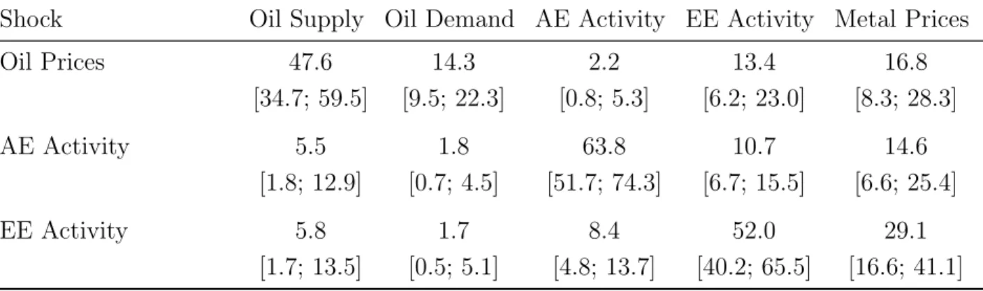
Table 5 shows the amount of variation in the two-year-ahead forecast error variance in oil prices, advanced economies’ IP and emerging economies’ IP that is attributable to the five structural shocks identified by our SVAR model. We choose to focus on the two-year horizon, as we consider it the typical horizon for business cycle analysis.28 _{As shown in the first row of table} ₅_{, about three-fourths of the} fluctuations in oil prices are due to shocks that originate in the oil market. In particular, shocks to oil supply account for more than 50 percent of the forecast error variance, while oil-specific demand shocks explain about 20 percent. Nonetheless, movements in global demand are a significant source of oil price fluctuations, explaining the remaining 25 percent of oil price fluctuations.29 _{Shocks to activity in} emerging economies and in metal prices are equally important drivers of oil prices, while the contribution of shocks to activity in advanced economies is almost zero.30

26_{Cashin et al.}₍₂₀₁₄_{) find that, following a supply-driven surge in oil prices, real activity falls in oil importing countries} and rises in net oil exporters, and that, following a global activity-driven oil demand shock, real activity increases for all economies in their sample regardless of their respective net oil trade patterns.

27_{The evidence in}_IMF₍_2015b_{) suggests that fluctuations in commodity prices and commodity terms-of-trade can lead} to sizable output fluctuations in commodity exporters, with this relationship particularly strong for exporters of energy and metals. Fernandez et al. (2015) also find support for the view that shocks to the prices of exported commodities explain a considerable portion of business cycle fluctuations in emerging economies. Furthermore, our findings are also consistent with those from the literature on emerging economies’ business cycle that terms-of-trade and world price shocks explain a significant fraction of cyclical fluctuations and that, in turn, variations in terms-of-trade are largely explained by variations in the prices of a few exported commodities. SeeMendoza(1995),Bidarkota and Crucini (2000),Kose(2002), andBaxter and Kouparitsas(2006).

28_{Results for the one-year-ahead forecast error variance decomposition are quantitatively similar.}

29_{Because the median contribution is calculated for each shock independently, the rows do not sum to 100 percent.} The medians of the total contributions to oil price fluctuations of oil-specific shocks and of global demand shocks are 72.2 percent and 25.3 percent, respectively.

30_{Stock and Watson} ₍₂₀₁₆_{) use factor models and find that the contribution of global demand shocks to oil price} fluctuations ranges between 20 and 40 percent, with their estimates reasonably close to our findings.

(19)

The second and third rows of table5show that, on average, oil-specific shocks contribute little to the volatility in real activity. Oil supply shocks account for about 5 percent of the forecast error variance of advanced economies’ and emerging economies’ IP, while the contribution of oil-specific demand shocks is a little below 2 percent in both advanced and emerging economies. Not surprisingly, activity variables are mostly driven by their own shocks. Yet, in line with the results from the forecast regressions, we find that shocks to metal prices, which are ordered last in our SVAR, account for 15 percent of the forecast error variance in advanced economies and for 30 percent in emerging economies.

Summing up, our results show that fluctuations in oil prices are primarily driven, on average, by oil supply shocks. In addition, movements in oil prices driven by global demand mostly reflect changes in oil demand from emerging economies, while they do not reflect changes in oil demand from advanced economies. We also find that oil shocks have a significant but secondary role in driving IP in both advanced and emerging economies, accounting for less than 10 percent of the variability at business cycle frequency.

4.4 Historical Decomposition

This section presents the historical decomposition of the actual paths of the VAR variables that is attributable to the oil market and global activity shocks.31 We first give an overview of the 1986–2015 period, presenting the data at an annual frequency. We then zoom in on three important episodes in the sample involving large changes in the price of oil. The first episode is centered on the Asian financial crisis, the second episode focuses on the period of the global financial crisis, and the third episode corresponds to the dramatic fall in the price of oil that started in July 2014 and lasts through the end of the sample. For these three episodes, we calculate the cumulative effects on each variable of shocks that materialized from the onset of the event onwards.32

Figure 6 shows the decompositions across the whole sample for the price of oil, oil production, and IP in both advanced economies and emerging economies. The black solid lines depict the actual paths of the VAR variables, whereas the areas colored in green, blue, cyan, red, and orange represent the contributions to the actual paths made by metal prices, advanced economies activity, emerging economies activity, oil supply, and oil demand shocks, respectively.

Overall, our results imply that, across the whole sample period, fluctuations in the price of oil and in oil production were mostly determined by shocks that are specific to the oil market, and in particular by supply shocks. Nonetheless, global activity contributed significantly to shaping fluctuations in oil

31_{We compute the historical decomposition using the OLS estimates of the reduced-form parameters. The sample used} for the estimation includes both actual data and the dummy observations used to implement the Minnesota prior.

32_{For these episodes, our decomposition sets previous shocks to zero, which explains why the vertical bars in figures}₇ to9,12, and13do not sum to the actual data depicted by the solid lines.

(20)

market variables. Shocks to emerging economies and to metal prices played a prominent role, while shocks to advanced economies activity played a modest role. Shocks emanating from the oil market contributed to fluctuations in advanced economies’ and emerging economies’ real activity. However, the quantitative importance of oil shocks, and, in particular, of oil supply shocks has varied considerably over the past three decades. Such shocks played an important role in the late 1990s and since 2012, but they had a distinctly secondary role in the remaining sample.

Although the aggregation to annual data offers a useful broad overview about the relative importance of the drivers in economic fluctuations, it misses some important aspects of the interaction between the oil market and macroeconomic variables that can be better revealed by appealing to a monthly narrative, which we discuss next for three episodes characterized by large swings in oil prices.

The Asian financial crisis. In figure 7, we plot the estimated historical decomposition of the model variables for the period of the Asian Financial Crisis from July 1997 to December 1998. All the panels display the change in the log of the variable since June 1997. The defining feature of this event was a sharp contraction in real activity in emerging economies, as shown in the lower-right panel. The decline in the demand of oil from emerging economies induced some downward pressure on oil prices and, if we include the contribution of shocks to metal prices, accounted for about one-third of the decline in oil prices.33

Throughout this period, despite a lower demand for oil from emerging countries, a few oil exporters, most notably Iraq, did not cut production and, on the contrary, increased production throughout early 1999. Accordingly, our model attributes a major role in the decline of the price of oil to supply shocks. Oil-specific demand shocks represented an offsetting factor for oil prices and, at the same time, account for about 15 percent of the increase in oil production in late 1997.

The effect of disturbances originated in the oil market on economic activity is positive but economi-cally small in advanced economies, while it is negative and more significant in emerging economies. The drop in oil prices caused by “excess production” in some oil-exporting countries resulted in a decline of almost 1 percent in emerging economies’ real activity.

The global financial crisis. In figure8, we plot the estimated historical decomposition of the model variables for the period of the global financial crisis from July 2008 to December 2009. All panels display the change in the log of the variable since June 2008. As indicated by the solid black line in the upper-left panel, the real price of oil experienced a dramatic plunge throughout this period. At the

33_{The narrative in}_{Baumeister and Kilian} ₍_2016a_{) attributes a large portion of the slide to reduced demand for crude} oil, arguably caused by the Asian financial crisis of mid-1997, which in turn was followed by economic crises in other countries including Russia, Brazil, and Argentina.

(21)

onset of the crisis, the model attributes much of the decline in the price of oil to negative oil-specific demand shocks, due to the simultaneous decline in oil production and the relatively small movements in global activity factors. The role of global activity shocks as drivers of the price of oil becomes more prominent toward the end of 2008, as the sharp decline in real activity materializes in both advanced and emerging economies.34

The model attributes some of the decline in the price of oil to positive supply shocks even though oil production is consistently below trend. Through the lens of the model, the sharp contraction in global activity at the end of 2008 should have led to an even larger reduction in oil production than that observed in the data. The higher-than-expected reading in oil production is rationalized by the model through the only shock that generates a negative co-movement between oil production and the price of oil, the oil supply shock.

The decomposition of the real activity variables plotted in the lower row of figure 8 provides a good reality check for the model. Consistent with the conventional wisdom, shocks originating in the oil market had nearly no role in the collapse of economic activity associated with the Great Financial Crisis.

The 2014–15 slump. Figure 9 displays the estimated historical decompositions for the July 2014– December 2015 period, characterized by a major slump in the real price of oil. All panels display the change in the log of the variable since June 2014. Throughout the episode, our identification attributes most of the decline in the price of oil to supply shocks. Oil-specific demand shocks contributed to the acceleration in the decline of the price of oil in early 2015. On the one hand, positive shocks to global supply, as detected by the decomposition of global production plotted in the upper-right panel, likely resulted from the enduring expansion in unconventional shale oil production, as also acknowledged by

Kilian(2016). On the other hand, the negative shocks to oil-specific demand were likely due to waning concerns about future availability of oil supplies and thus heightened expectations of future excess supply in global oil markets. These expectations, in turn, presumably reflected a few main factors—for instance, the return to production of oil fields in Iraq and Libya following the end of military threats from extremists, greater market confidence that the expansion in shale oil production would not suddenly lose momentum following the price slump, and OPEC’s unwillingness to cut production and thus follow through with a policy of stabilizing prices, as typically done in earlier decades.35 _{Since early 2015,}

34_{Our characterization of the plunge in oil prices is in line with the results in}_{Juvenal and Petrella}₍₂₀₁₅_{), who found} that the collapse was explained mostly by a negative speculative shock, as the financial crisis hurt the balance sheets of many financial investors, and by a negative supply shock, mainly reflecting the recession after the financial crisis.

35_{Even though many commentaries remarked that the decision of OPEC to keep its production target unchanged was} largely anticipated, between the end of November and the beginning of December in 2014—that is, in the days immediately following OPEC’s decision—the Brent price of oil lost a remarkable amount of about $5 per barrel.

(22)

the decline in the price of oil also began to reflect negative shocks both in emerging economies and to expectations of global activity as captured by the shock to metal prices.36

As shown in the lower row of figure9, oil shocks had no role in shaping economic activity in advanced economies until mid-2015. Since June 2015, oil supply shocks have added about 1 percent to growth in industrial production in advanced economies. On the contrary, oil shocks were part of the headwinds faced by emerging economies since late 2014. The contribution to the decline in industrial output was a little over 0.1 percent as of October 2014, rising subsequently to about 1 percent at the end of 2015. The boost in economic activity in advanced economies in conjunction with the drag on economic activity in emerging economies of about equal size thus rationalizes the muted response of global activity to oil market developments.

4.5 Summary of Findings

All told, the analysis in this section shows that (1) under our identification, oil supply and oil-specific demand shocks induce significant movements in oil prices and quantities; (2) shocks to global demand account, on average, for about 25 percent of fluctuations in oil prices, and are important drivers of oil prices during some historical episodes; and (3) shocks that originate in the oil market have asymmetric effects on activity in advanced and emerging economies but are not important contributors to business cycle fluctuations in global real activity.

5 The Role of Oil Price Elasticities

In this section we analyze the sensitivity of our results to changes in the assumptions about the oil supply elasticity. We present the results by discussing the effect of changes in the oil supply elasticity because most of the literature has focused on this structural parameter and, as we have shown in Section3, there is a one-to-one relationship between the oil supply and oil demand elasticities. We first show how small differences in the oil supply elasticity can change the sign of the predicted effects on economic activity of shocks originating in the oil market. We then show how different assumption about the elasticity change the share of the variance of oil and activity variables explained by the various shocks. Moreover, we show how changes in the oil supply elasticity affect the inference about the driving forces of oil prices during two episodes of large oil price movements. This exercise also highlights how the use of multiple

36_{The gap between the vertical bars and the black line in the upper-left panel of figure}₉ _{shows that about 30 percent} of the decline in oil prices was actually predictable, as it reflected the cumulative effects of earlier shocks. Baumeister and Kilian(2016b) find that this predictable component is more than 50 percent. They also find that the unpredictable portion of the price decline is not related to supply disturbances but instead reflects a negative shock to oil price expectations in July 2014 and a shock to the demand for oil in December 2014 primarily originating from emerging economies.

(23)

indicators of global demand for oil is instrumental toward the goal of disentangling oil market-specific shocks and global demand shocks.

5.1 Global Effects of Oil Market Shocks

Figure 10 illustrates the importance of selecting among alternative oil supply elasticities in order to gauge the aggregate effects of shocks originating in the oil market. To make our point, we consider the hypothetical question of how economic activity would respond to a 1 percent change in the price of oil. In particular, the upper panel plots the two-year elasticity of IP in advanced economies to oil prices changes driven by oil supply shocks (the red solid line) and by oil-specific demand shocks (the blue dashed line) as a function of the oil supply elasticity. Similarly, the lower panel plots the corresponding two–year elasticity of IP in emerging economies.

Under our benchmark identification scheme (shown by the vertical line corresponding toη_S = 0.11), a 1 percent rise in oil prices driven by an oil supply shock leads to a 0.04 percent drop in advanced economies’ IP and to a 0.03 percent rise in emerging economies’ IP. By contrast, the same oil price rise, when driven by shocks to oil demand, has more muted effects on activity in advanced economies, even as its effects on emerging economies are roughly unchanged. This result suggests that oil-specific demand shocks capture, at least in part, higher demand for energy-intensive goods (such as cars or heavy equipment) driven by better growth prospects in emerging economies.

The upper panel shows that as the oil supply elasticity rises (and, consequently, the oil demand elasticity falls), the VAR predicts more benign effects on activity in advanced economies from oil– market driven changes in oil prices. For instance, the IP elasticity evaluated at η_S = 0, the value used in Kilian (2009), is -0.1, twice as large as under our identification. By contrast, as shown in the lower panel, as the oil supply elasticity rises, supply-driven increases in oil prices have more positive effects on emerging economies’ activity, whereas demand-driven increases in oil prices have more negative effects.

5.2 Oil Price Elasticities and Volatilities

Figure 11 plots the share of the variance of the two-year-ahead forecast errors for oil prices, IP in advanced economies, and IP in emerging economies that is attributable to oil shocks as a function of the supply elasticity. The red solid line plots the contribution of oil supply shocks, the blue solid line plots the contribution of oil-specific demand shocks, and the black dashed line plots their sum. The remaining share of variability is due to global activity shocks.

The left panel of figure11shows the forecast error variance decomposition for oil prices. The relative importance of oil-specific demand and supply shocks changes considerably as the oil supply elasticity

(24)

varies. As reported in table5, according to our benchmark identification scheme (shown by the vertical line), oil-specific shocks explain about 65 percent of the two–year forecast error variance of oil prices, with oil supply shocks accounting for the largest share, about 50 percent. By contrast, if the supply elasticity were close to zero, oil supply shocks would explain none of the oil–market driven volatility in prices, and, if the supply elasticity were to rise to 0.2, would explain nearly all of the oil–market driven volatility in prices. On the contrary, the assumption on the oil supply elasticity has only a minor effecxt on the overall share of volatility that is explained by oil shocks, which rises from 65 percent for a supply elasticity equal to zero to 70 percent for a supply elasticity equal to 0.2.

The middle and right panels of figure 11 show the share of two-year-ahead volatility in advanced economies’ and emerging economies’ activity that is explained by oil market shocks, again as a function of the oil supply elasticity. As the two panels show, while the relative importance of oil demand and oil supply shocks changes considerably as the oil supply elasticity varies, the overall share of volatility in advanced and emerging economies that is explained by oil shocks is small regardless of the value of elasticity, ranging between 5 and 10 percent. Nonetheless, and in line with the comparison of the IP elasticities to oil prices, we find that an increase in the oil supply elasticity decreases the share of fluctuations in advanced economies’ IP explained by oil market-specific shocks, whereas it increases the share of fluctuations in emerging economies’ IP generated by the oil shocks.

5.3 Oil Price Elasticities and the Decoupling Puzzle

Figures 12 and 13 compare the historical decomposition for oil prices and oil production during the Asian financial crisis and the 2014–15 oil slump obtained with three different specifications of the SVAR model.

Panel A in figure 12 reproduces the historical decomposition of the Asian financial crisis under our identification scheme. As already discussed, our decomposition is characterized by (1) the joint movement in oil prices and oil production induced by positive oil supply shocks, and (2) the importance of the decline in emerging economies activity in accounting for the decline in oil prices. By contrast, panel B shows how a model with zero oil supply elasticity requires positive oil supply shocks to explain the rise in oil production and negative oil demand shocks to explain the fall in oil prices. That is, the zero supply elasticity model decouples fluctuations in oil supply and oil demand shocks. Finally, panel C shows the results of a SVAR that retains the zero oil supply elasticity but replaces the three global activity indicators with Kilian (2009)’s real global activity index. The comparison between panels A and C illustrates the difference between our global activity indicators and Kilian (2009)’s index. It is remarkable how such an index fails to find any connection between the sharp slowdown in emerging economies activity and the concurrent decline in oil prices.