Automatic Virtual Machine Configuration for Database
Workloads
Ahmed A. Soror
†∗Umar Farooq Minhas
†Ashraf Aboulnaga
†Kenneth Salem
†Peter Kokosielis
‡Sunil Kamath
‡†
University of Waterloo ‡
IBM Toronto Lab †
{aakssoro, ufminhas, ashraf, kmsalem}@cs.uwaterloo.ca ‡
{pkolosie, sunil.kamath}@ca.ibm.com
ABSTRACT
Virtual machine monitors are becoming popular tools for the deployment of database management systems and other enterprise software applications. In this paper, we consider a common resource consolidation scenario, in which several database management system instances, each running in a virtual machine, are sharing a common pool of physical com-puting resources. We address the problem of optimizing the performance of these database management systems by con-trolling the configurations of the virtual machines in which they run. These virtual machine configurations determine how the shared physical resources will be allocated to the different database instances. We introduce a virtualization design advisor that uses information about the anticipated workloads of each of the database systems to recommend workload-specific configurations offline. Furthermore, run-time information collected after the deployment of the rec-ommended configurations can be used to refine the recom-mendation. To estimate the effect of a particular resource allocation on workload performance, we use the query opti-mizer in a new what-if mode. We have implemented our ap-proach using both PostgreSQL and DB2, and we have exper-imentally evaluated its effectiveness using DSS and OLTP workloads.
Categories and Subject Descriptors
H.2.2 [Database Management]: Physical Design
General Terms
Algorithms, Design, Experimentation, Performance
Keywords
Virtualization, Virtual Machine Configuration, Resource Con-solidation
∗
Supported by an IBM CAS Fellowship.
Permission to make digital or hard copies of all or part of this work for personal or classroom use is granted without fee provided that copies are not made or distributed for profit or commercial advantage and that copies bear this notice and the full citation on the first page. To copy otherwise, to republish, to post on servers or to redistribute to lists, requires prior specific permission and/or a fee.
SIGMOD’08,June 9–12, 2008, Vancouver, BC, Canada. Copyright 2008 ACM 978-1-60558-102-6/08/06 ...$5.00.
1.
INTRODUCTION
Virtual machine monitors are becoming popular tools for the deployment of database management systems and other enterprise software systems. Virtualization adds a flexible and programmable layer of software between “applications”, such as database management systems, and the resources used by these applications. This layer of software, called the virtual machine monitor (VMM), maps the virtual re-sources perceived by applications to real physical rere-sources. By managing this mapping from virtual resources to phys-ical resources and changing it as needed, the VMM can be used to transparently allow multiple applications to share resources and to change the allocation of resources to appli-cations as needed.
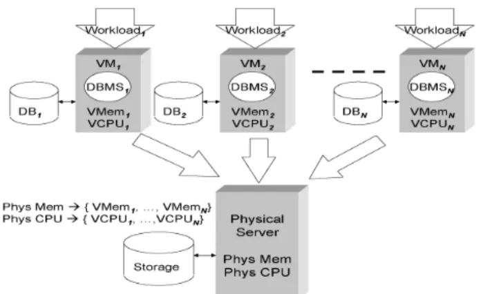
There are many reasons for virtualizing resources. For example, some virtual machine monitors enable live migra-tion of virtual machines (and the applicamigra-tions that run on them) among physical hosts. This capability can be ex-ploited, for example, to simplify the administration of phys-ical machines or to accomplish dynamic load balancing. One important motivation for virtualization is to support enter-priseresource consolidation. Resource consolidation means taking a variety of applications that run on dedicated com-puting resources and moving them to a shared resource pool. This can improve the utilization of the physical resources, simplify resource administration, and reduce cost for the en-terprise. One way to implement resource consolidation is to place each application in a virtual machine (VM) which en-capsulates the application’s original execution environment. These VMs can then be hosted by a shared pool of physical computing resources. This is illustrated in Figure 1.
When creating a VM for one or more applications, it is important to correctly configure this VM. One of the most important decisions when configuring a VM is deciding how much of the available physical resources will be allocated to this VM. Our goal in this paper is to automatically make this decision for virtual machines that host database manage-ment systems and compete against each other for resources. As a motivating example, consider the following scenario, We created two Xen [2] VMs, each running an instance of PostgreSQL, and hosted them on the same physical server.1 On the first VM, we run a workload consisting of 1 copy of TPC-H query Q17 on a 10GB database. We call this Workload 1. On the second VM, we run a workload on an
1The full details of our experimental setup can be found in
Figure 1: Resource consolidation using virtual ma-chines.
Figure 2: Motivating example.
identical 10GB TPC-H database consisting of 132 copies of a modified version of TPC-HQ18 (we modified the sub-query inQ18 so that it touches less data). We call this Workload 2. As an initial configuration, we allocate 50% of the available CPU capacity to each of the two VMs. When we apply our configuration technique, it recommends allocating 20% of the available CPU capacity to the VM running Workload 1 and 80% to the VM running Workload 2. Figure 2 shows the execution time of the two workloads under the initial and recommended configurations. Workload 1 suffers a slight degradation in performance (4%) under the recommended configuration as compared to the initial configuration. On the other hand, the recommended configuration boosts the performance of Workload 2 by 34%. This is because Work-load 1 is very I/O intensive in our execution environment, so its performance is not sensitive to changes in CPU al-location. Workload 2, in contrast, is CPU intensive, so it benefits from the extra CPU allocation. This simple exam-ple illustrates the potential performance benefits that can be obtained by adjusting resource allocation levels based on workload characteristics.
Our approach to virtual machine configuration is to use in-formation about the anticipated workloads of each database management system (DBMS) to determine an appropriate configuration for the virtual machine in which it runs. An advantage of this approach is that we can avoid allocating resources to DBMS instances that will obtain little benefit from them. For example, we can distinguish CPU intensive
workloads from I/O intensive workloads and allocate more CPU to the former. Our technique is implemented as a vir-tualization design advisor, analogous to the physical design advisors currently available for most relational DBMS. How-ever, our virtualization design advisor differs from DBMS physical design advisors in two significant ways. First, it recommends a configuration for the virtual machine con-taining the DBMS, rather than the DBMS itself. Second, our advisor is used to recommend configurations for a set of virtual machines that are sharing physical resources, while most DBMS physical design tools guide the configuration of a single DBMS instance. Once the configured virtual ma-chines are up and running, our advisor is also capable of collecting runtime information that allows it to refine its recommendations online.
The rest of this paper is organized as follows. Section 2 presents an overview of related work. In Section 3, we present a definition of the virtualization design problem. Section 4 describes our virtualization design advisor and presents a cost model calibration methodology that allows the design advisor to leverage the query optimizer cost mod-els of the DBMSes that are being consolidated. In Section 5, we present an extension to the advisor that allows it to refine its recommendations using runtime performance measure-ments of the consolidated, virtualized DBMS instances. In Section 6, we present an experimental evaluation of our ap-proach using PostgreSQL and DB2 as our target DBMSes. We conclude in Section 7.
2.
RELATED WORK
There are currently several technologies for machine vir-tualization [2, 14, 17, 23], and our proposed virvir-tualization design advisor can work with any of them. As these virtu-alization technologies are being more widely adopted, there is increasing interest in the problem of automating the de-ployment and control of virtualized applications, including database systems [9, 15, 16, 19, 24, 25]. Work on this prob-lem varies in the control mechanisms that are exploited and in the performance modeling methodology and optimization objectives that are used. However, a common feature of this work is that the target applications are treated as black boxes that are characterized by simple models, typically gov-erned by a small number of parameters. In contrast, the vir-tualization design advisor described in this paper is specific to database systems, and it attempts to exploit database system cost models to achieve its objectives. There is also work on application deployment and control, including re-source allocation and dynamic provisioning, that does not exploit virtualization technology [3, 8, 21, 22]. However, this work also treats the target applications as black boxes.
The virtualization design problem that is considered here was posed, but not solved, in our previous work [18]. This paper builds on that previous work by proposing a complete solution to the problem in the form of a virtualization design advisor. We also incorporate quality of service constraints into the problem definition, and we present an empirical evaluation of the proposed solution.
There has been a substantial amount of work on the prob-lem of tuning database system configurations for specific workloads or execution environments [26] and on the prob-lem of making database systems more flexible and adap-tive in their use of computing resources [1, 6, 10, 12, 20]. However, in this paper we are tuning the resources to the
database system, rather than the other way around. Re-source management and scheduling have also been addressed within the context of database systems [4, 5, 7, 11]. That work focuses primarily on the problem of allocating a fixed pool of resources to individual queries or query plan op-erators, or on scheduling queries or operators to run on the available resources. In contrast, our resource alloca-tion problem is external to the database system, and hence our approach relies only on the availability of query cost estimates from the database systems.
3.
PROBLEM DEFINITION
Our problem setting is illustrated in Figure 1. N virtual machines, each running an independent DBMS, are com-peting for a pool of physical resources. For each DBMS, we are given a workload description consisting of a set of SQL statements (possibly with a frequency of occurrence for each statement). We useWi (1≤i≤N) to represent the
work-load of theith DBMS. In our problem setting, since we are making resource allocation decisions across workloads and not for one specific workload, it is important that the work-loads represent the statements processed by the different DBMSesin the same amount of time. Thus, a longer work-load represents a higher rate of arrival for SQL statements. We assume that there are M different types of physical resources, such as memory, CPU capacity, or I/O band-width, that are to be allocated to the virtual machines. Our problem is to allocate a share, or fraction, of each physi-cal resource to each of the virtual machines. We will use
Ri = [ri1, . . . , riM], 0 ≤rij ≤1, to represent the resource
shares allocated to workload Wi’s virtual machine. The
shares are used to set configuration parameters in the vir-tual machines so that the resource allocations described by the shares are enforced by the virtual machine monitor.
We assume that each workload has an associated cost, which depends on the resources allocated to the virtual ma-chine in which the workload runs. We useCost(Wi, Ri) to
represent the cost of workloadWiunder resource allocation
Ri. Our goal is to find a feasible set of resource
alloca-tionsrij such that the total cost over all of the workloads
is minimized. Specifically, we must chooserij (1≤i≤N,
1≤j≤M) such that
N
X
i=1
Cost(Wi, Ri)
is minimized, subject torij≥0 for alli, jandPNi=1rij= 1
for all j. This problem was originally defined (but not solved) in [18], and was named the virtualization design problem.
In this paper, we have also considered a constrained ver-sion of the virtualization design problem. The constrained version is identical to the original problem, except for an additional requirement that the solution must satisfy qual-ity of service (QoS) requirements imposed on one or more of the workloads. The QoS requirements specify the maximum increase in cost that is permitted for a workload under the chosen resource assignment. We define thecost degradation
for a workloadWiunder a resource assignmentRi as
Degradation(Wi, Ri) =
Cost(Wi, Ri)
Cost(Wi,[1, . . . ,1])
where [1, . . . ,1] represents the resource assignment in which
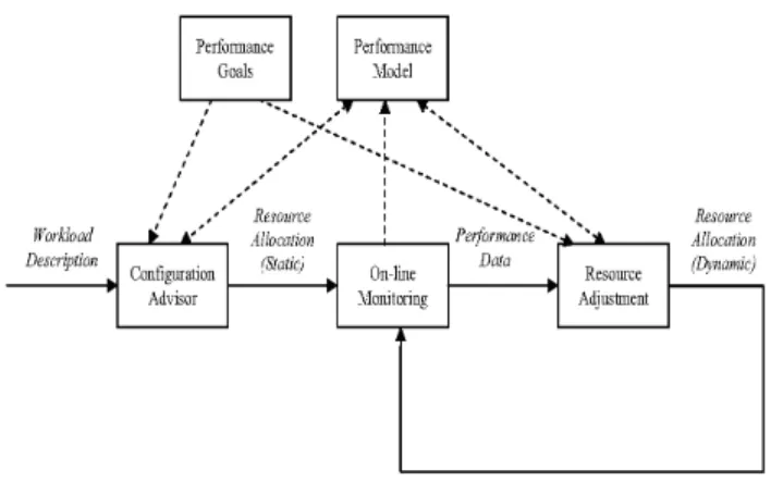
Figure 3: Virtualization design advisor.
all of the available resources are allocated to Wi. In the
constrained version of the virtualization design problem, a
degradation limitLi is specified for each workloadWi, and
the solution is required to obey the constraint
Degradation(Wi, Ri)≤Li
for all workloads. The degradation limitLican be specified
to be infinite for workloads for which limiting degradation is not desired.
We also introduce a mechanism for specifying relative pri-orities among the different workloads. Abenefit gain factor
Gican be specified for each workload, indicating how
impor-tant it is to improve the performance of this workload com-pared to other workloads. Each unit of cost improvement for the workload is considered to be worth Gicost units. The
default setting for the different workloads isGi= 1,
indicat-ing that all workloads should be treated equally. Increasindicat-ing
Gifor a particular workload may cause it to get more than
its fair share of resources since cost improvements to it are amplified. Incorporating this metric into our problem defini-tion requires us to change the cost equadefini-tion being minimized to the following:
N
X
i=1
Gi×Cost(Wi, Ri)
In this paper, we focus on the case in which the two re-sources to be allocated among the virtual machines are CPU time and memory, i.e.,M = 2. Most virtual machine moni-tors currently provide mechanisms for controlling the alloca-tion of these two resources to VMs, but it is uncommon for virtual machine monitors to provide mechanisms for control-ling other resources, such as storage bandwidth. Neverthe-less, our problem formulation and our virtualization design advisor can handle as many resources as the virtual machine monitor can control.
4.
VIRTUALIZATION DESIGN ADVISOR
A high level overview of our virtualization design advisor is given in Figure 3. The advisor makes initial, static re-source allocation recommendations based on the workload descriptions and performance goals. Two modules within the design advisor interact to make these recommendations: a configuration enumerator and a cost estimator. The con-figuration enumerator is responsible for directing the explo-ration of the space of possible configuexplo-rations, i.e., allocations
Parameter Description
random page cost cost of non-sequential disk page I/O
cpu tuple cost CPU cost of processing one tu-ple
cpu operator cost per-tuple CPU cost for each WHERE clause
cpu index tuple cost CPU cost of processing one in-dex tuple
shared buffers shared database bufferpool size work mem amount of memory to be used by sorting and hashing opera-tors
effective cache size size of the file system’s page cache
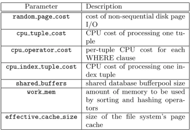
Figure 4: PostgreSQL optimizer parameters.
of resources to virtual machines. The configuration enumer-ator is described in more detail in Section 4.3. To evaluate the cost of a workload under a particular resource allocation, the advisor uses the cost estimation module. Given a work-loadWiand a candidate resource assignmentRi, selected by
the configuration enumerator, the cost estimation module is responsible for estimatingCost(Wi, Ri). Cost estimation is
described in more detail in Section 4.1.
In addition to recommending initial virtual machine con-figurations, the virtualization design advisor can also adjust its recommendations dynamically based on observed work-load costs to correct for any cost estimation errors at the original recommendation phase. This online refinement is described in Section 5.
4.1
Cost Estimation
Given a workload Wi and a candidate resource
alloca-tion Ri, the cost estimator is responsible for estimating
Cost(Wi, Ri). Our strategy for cost estimation is to leverage
the cost models that are built into the database systems for query optimization. These models incorporate a wealth of information about query processing within the DBMS, and we would like to avoid reinventing this for the purpose of virtualization design.
A DBMS cost model can be described as a function
CostDB(Wi, Pi, Di), where Wi is a SQL workload, Pi =
[pi1, pi2, . . . , PiL] is a vector of optimizer configuration
pa-rameters, andDiis the database instance. The parameters
Pi are used to describe both the available computing
re-sources and relevant parts of the DBMS configuration to the cost model. For example, Figure 4 lists the relevant configuration parameters used by PostgreSQL version 8.1.3. There are two difficulties in directly applying the DBMS cost model for cost estimation for virtualization design. The first problem is the difficulty of comparing cost estimates produced by different DBMSes. This is required for vir-tualization design because the design advisor is required to assign resources to multiple database systems, each of which may use a different cost model. DBMS cost models are in-tended to produce estimates that can be used to compare the costs of alternative query execution strategies for a single DBMS and a fixed execution environment. In general, com-paring cost estimates from different DBMS may be difficult because they may have very different notions of cost. For
Figure 5: Cost estimation for virtualization design.
example, one DBMS’s definition of cost might be response time, while another’s may be total computing resource con-sumption. Even if two DBMSes have the same notion of cost, the cost estimates are typically normalized, and dif-ferent DBMSes may normalize costs difdif-ferently. The first of these two issues is beyond the scope of this paper, and fortunately it is often not an issue since many DBMS opti-mizers define cost as total resource consumption. For our purposes we will assume that this is the case. The normal-ization problem is not difficult to solve, but it does require that we renormalize the result ofCostDB(Wi, Ri, Di) so that
estimates from different DBMS will be comparable. The second problem is that the DBMS cost estimates de-pend on the parametersPi, while the virtualization design
advisor is given a candidate resource allocationRi. Thus, to
leverage the DBMS query optimizer, we must have a means of mapping the given candidate resource allocation to a set of DBMS configuration parameter values that reflect the candidate allocation. We use this mapping to define a new “what-if” mode for the DBMS query optimizer. Instead of generating cost estimates under fixed settings ofPi, we map
a givenRito the correspondingPi, and we use thePito
an-swer the question: “ifthe parameter settings were to be set in a particular way, what would be the cost of the optimal plan for the given workload?”.
To address these problems, we construct cost estimators for virtualization design as shown in Figure 5. A calibra-tion step is used to determine a set of DBMS cost model configuration parameters corresponding to the given candi-date resource allocation Ri. Once these parameter values
have been set, the DBMS cost model is then used to gen-erate CostDB for the given workload. Finally, this cost is
renormalized to produce the cost estimate required by the virtualization design advisor.
The calibration and renormalization steps shown in Fig-ure 5 must be custom-designed for each type of DBMS for which the virtualization design advisor will be recommend-ing designs. To test the feasibility of this approach, we have designed calibration and renormalization steps for both PostgreSQL and DB2. In the following, we describe how these steps were designed, using PostgreSQL as an illustra-tive example. The methodology for DB2 is very similar.
As has already been noted, we assume that the DBMS defines cost as total resource consumption and, as a result, the renormalization step is simple. For example, in Post-greSQL, all costs are normalized with respect to the time required for a single sequential I/O operation. We have chosen to express costs in units of seconds. Thus,
renor-malization for PostgreSQL simply requires that we multiply
CostDBby the number of seconds required for a sequential
I/O operation. To determine this renormalization factor, we created a simple calibration program that sequentially reads 8 kilobyte (the PostgreSQL page size) blocks of data from the virtual machine’s file system and reports the average time per block.
The calibration of the optimizer configuration parameters
Pi is more involved. We can distinguish two types of
pa-rameters. Prescriptive parameters define the configuration of the DBMS itself. Changing the value of these param-eters changes the configuration of the DBMS itself. For PostgreSQL,shared buffersandwork memare prescriptive parameters. Descriptive parameters, in contrast, exist only to characterize the execution environment. Changing these parameters affects the DBMS only indirectly through the effect that they have on cost estimates. In PostgreSQL, parameters like cpu tuple cost, random page cost, and effective cache sizeare descriptive parameters.
Values for prescriptive parameters must be chosen to re-flect the mechanisms or policies that determine the DBMS configuration. For example, if the PostgreSQL work mem parameter will be left at its default value regardless of the amount of memory that our design advisor allocates to the virtual machine in which the DBMS will run, then the calibration procedure should simply assign that default value to the work mem parameter. If, on the other hand, the DBMS’s configuration will be tuned in response to the amount of memory that is allocated to the virtual machine, then the calibration procedure should model this tuning pol-icy. For example, in our experiments our policy was to setshared buffersto 1/16 of the memory available in the host virtual machine, and to setwork memto 5MB regardless of the amount of memory available. Thus, our calibration procedure mimics these policies, settingshared buffers ac-cording to the virtual machine memory allocation described byRi and settingwork memto 5MB regardless ofRi.
For each descriptive parameterpik, we wish to determine
a calibration functionCalik that will define a value forpik
as a function of the candidate resource allocationRi. To
do this, we use the following basic methodology for each parameterpik:
1. Define acalibration queryQand acalibration database
D such that CostDB(Q, Pi, D) is independent of all
descriptive parameters inPiexcept forpik.
2. Choose a resource allocation Ri, instantiate D, and
runQunder that resource allocation, and measure its execution timeTQ.
3. Solve Renormalize(CostDB(Q, Pi, D)) = TQ for pik,
and associate the resultingpikvalue with the resource
allocationRi. Here theRenormalize() function
rep-resents the application of the renormalization factor that was determined for the DBMS.
4. Repeat the two preceding steps for a variety of different resource allocationsRi, associating each with a value
ofpik.
5. Perform regression analysis on the set of (Ri, pik) value
pairs to determine calibration functionCalik from
re-source allocations topik values.
A specific instance of this general methodology must be designed for each type of DBMS that will be considered by the virtualization design advisor. The primary design tasks are the design of the calibration queriesQand calibra-tion databaseD (Step 1), the choice of resource allocations for which calibration measurements will be taken (Step 2), and the choice of function to be fit to the calibration data (Step 5). The design of the calibration methodology de-mands deep expertise in the implementation of the target DBMS for the selection of calibration queries and database in Step 1. For example, it is important to ensure that the cost of the calibration queries is dependent only on the pa-rameter that is being calibrated. It is also important to choose the calibration database in such a way that all opti-mizer assumptions are satisfied, so that the cost estimates it produces are accurate. For example, if the optimizer assumes a uniform data distribution then the calibration database should be uniformly distributed. The expertise re-quired for designing the calibration methodology is not a major constraint on our approach, since this methodology need only be designed once for each type of DBMS.
In practice, the basic methodology can be refined and gen-eralized in several ways. One improvement is to choose cal-ibration queries in Step 1 that have minimal non-modeled
costs. For example, one cost that is typically not modeled is the cost of returning the query result to the application.2 This cost can be minimized by choosing calibration queries that return few rows. Care is also required in defining the calibration database. For example, it should be just large enough to allow query execution times to be measured ac-curately. Larger databases will increase the run times of the calibration queries and hence the cost of calibration. Ideally, a single calibration database would be designed to be shared by all of the calibration queries so that it is not necessary to instantiate multiple databases during calibration.
Another potential problem with the basic methodology is that it may not be possible to choose a single query that isolates a particular cost model parameter in Step 1. In this case, one can instead identify a set of k queries that de-pend on k parameters (only). In Step 3 of the algorithm, a system of k equations is solved to determine values for thek parameters for a given resource allocation. As a sim-ple examsim-ple, consider the design of a calibration method for thecpu tuple costparameter. PostgreSQL models the cost of a simple sequential table scan as a linear function of cpu tuple cost that involves no other cost model pa-rameters. Thus, we could use a simple single-table selec-tion query without predicates as our calibraselec-tion query for cpu tuple costin Step 1. However, such a query would po-tentially return many tuples, leading to a large unmodeled cost. To eliminate this problem, we could instead choose a select count(*)query without predicates, since such a query will return only a single row. However, the use of aggregation in the query introduces a second cost model parameter (cpu operator cost) into the query cost model. Thus, a second calibration query involving the same two pa-rameters will be required. One possibility is to use another select count(*)query with agroup byclause. The mea-sured run times of these two queries will then define a system of two equations that can be solved to determine
appropri-2
DBMS cost models ignore this cost because it is the same for all plans for a given query, and thus is irrelevant for the task of determining which plan is cheapest.
Figure 6: Variation in cpu tuple cost.
Figure 7: Variation incpu operator cost.
ate values for cpu operator cost and cpu tuple cost for each tested resource allocation.
4.2
Optimizing the Calibration Process
One of our major concerns was “How can we reduce the number of different virtual machines we need to realize and the number of calibration queries we need to run in order to calibrate the query optimizer?” If we haveN CPU settings andM memory settings for the calibration experiments, a simplistic approach would be to realizeN×M virtual ma-chines and calibrate the parameters for each one. However, we could significantly reduce the calibration effort by relying on the observation that CPU, I/O, and memory optimizer parameters areindependentof each other and hence can be calibrated independently. We have verified this observation experimentally on PostgreSQL and DB2.
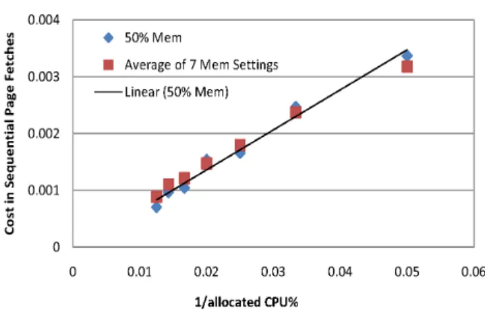
For example, we have observed that the PostgreSQL CPU optimizer parameters vary linearly with 1/(allocated CPU fraction). This is expected since if the CPU share of a VM is doubled, its CPU costs would be halved. At the same time, the CPU parameters do not vary with memory since they are not describing memory. Thus, instead of needing
N×M experiments to calibrate CPU parameters, we only needN experiments for the N CPU settings. Figures 6–8 show the linear variation of the three CPU parameters of the PostgreSQL optimizer with 1/(CPU share). The fig-ures show for each parameter the value of the parameter obtained from a VM that was given 50% of the available
Figure 8: Variation incpu index tuple cost.
Figure 9: Objective function for two workloads not competing for CPU.
memory, the average value of the parameter obtained from 7 different VMs with memory allocations of 20%–80%, and a linear regression on the values obtained from the VM with 50% of the memory. We can see from the figures that CPU parameters do not vary too much with memory, and that the linear regression is a very accurate approximation. Thus, in our calibration of PostgreSQL, we calibrate the CPU pa-rameters at 50% memory allocation, and we use a linear regression to model how parameter values vary with CPU allocation. We have found similar optimization opportuni-ties for memory parameters, which can be calibrated at one CPU setting, and I/O parameters, which do not depend on CPU or memory and can be calibrated once.
We expect that for all database systems, the optimizer pa-rameters describing one resource will be independent of the level of allocation of other resources, and we will be able to optimize the calibration process as we did for PostgreSQL. This requires expert knowledge of the DBMS, but it can be considered part of designing the calibration process for the DBMS, which is performed once by the DBMS expert and then used as many times as needed by users of the virtual-ization design advisor.
4.3
Configuration Enumeration
The shape of the objective function we are minimizing is fairly smooth and concave. For example, Figures 9 and 10 show the shape of this function for two workload mixes from the TPC-H benchmark running on PostgreSQL. In Figure 9,
Figure 10: Objective function for two workloads competing for CPU.
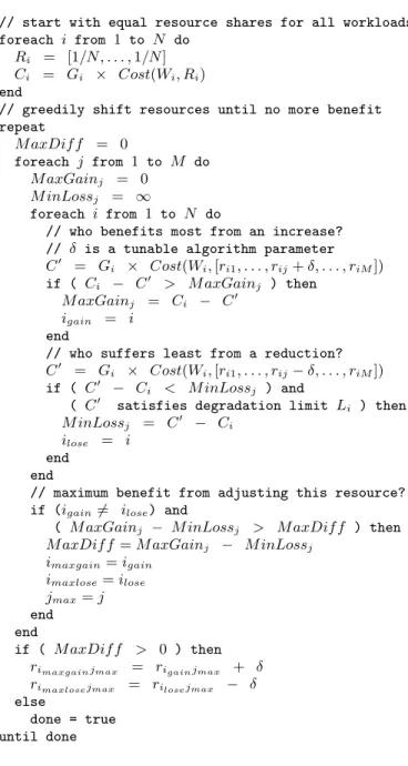
// start with equal resource shares for all workloads foreach i from 1 to N do
Ri = [1/N , . . . ,1/N]
Ci = Gi × Cost(Wi, Ri)
end
// greedily shift resources until no more benefit repeat M axDif f = 0 foreach j from 1 to M do M axGainj = 0 M inLossj = ∞ foreach i from 1 to N do
// who benefits most from an increase? // δ is a tunable algorithm parameter
C0 = Gi × Cost(Wi,[ri1, . . . , rij+δ, . . . , riM])
if ( Ci − C0 > M axGainj ) then
M axGainj = Ci − C0
igain = i
end
// who suffers least from a reduction?
C0 = Gi × Cost(Wi,[ri1, . . . , rij−δ, . . . , riM])
if ( C0 − Ci < M inLossj ) and
( C0 satisfies degradation limit Li ) then
M inLossj = C0 − Ci
ilose = i
end end
// maximum benefit from adjusting this resource? if (igain6= ilose) and
( M axGainj − M inLossj > M axDif f ) then
M axDif f =M axGainj − M inLossj
imaxgain=igain imaxlose=ilose jmax=j end end if ( M axDif f > 0 ) then
rimaxgainjmax = rigainjmax + δ
rimaxlosejmax = rilosejmax − δ else
done = true until done
Figure 11: Greedy configuration enumeration.
one workload is CPU intensive and the other is not, and in Figure 10 both workloads are CPU intensive and are com-peting for CPU. In both cases the shape of the cost function remains smooth and concave. We have also verified this for the case where we haveN >2 workloads. Hence, we adopt agreedy searchas our search algorithm. Due to the nature of the objective function, greedy search is accurate and fast, and is not likely to terminate at a local minimum. We have observed that when the greedy search does terminate at a local minimum, this minimum is not far off from the global minimum.
Figure 11 illustrates our greedy configuration enumera-tion algorithm. Initially, the algorithm assigns a 1/N share of each resource to each of the N workloads. It then pro-ceeds iteratively. In each iteration, it considers shifting a share δ (say, 5%) of some resource from one workload to another. The algorithm considers all such resource reallo-cations, and if it finds reallocations of resources that are beneficial according to the cost estimator, then it makes the most beneficial reallocation and iterates again. If no benefi-cial reallocations are found, algorithm terminates, reporting the current resource allocations as the recommended alloca-tions.
The algorithm is greedy in the sense that it always re-moves resources from the workload whose estimated cost will increase the least as a result of the reallocation, and always adds resources to the workload whose estimated cost will decrease the most as a result. If a workload has a per-formance degradation limit,Li, the algorithm will only take
resources away from this workload if its performance after its resource level is reduced still remains within its degra-dation limit. If a workload has a benefit gain factor, Gi,
the algorithm will multiply its cost by Gi for all levels of
resource allocation. Since each iteration’s reallocation af-fects only two workloads and the reallocation only occurs if those workloads see a combined net cost reduction, each iteration of the algorithm will decrease the total cost of the
N workloads.
Unlike the cost model calibration procedure described in Section 4.1, the greedy search algorithm used for configura-tion enumeraconfigura-tion does not require any access to the virtual-ization infrastructure and does not involve the execution of any database queries, since it is based on cost models. The algorithm does, however, call the DBMS query optimizer to estimate costs, and these calls can potentially be expensive. A simple way to reduce the number of optimizer calls is to cache the estimated costs computed in one iteration of the algorithm and reuse them in subsequent iterations. Since the algorithm changes the resource allocation of only two workloads in each iteration, there will be lots of opportuni-ties for reusing cached costs.
5.
ONLINE REFINEMENT
Our virtualization design advisor relies for cost estima-tion on the query optimizer calibrated as described in the previous section. This enables the advisor to make resource allocation recommendations based on an informed and fairly accurate cost model without requiring extensive experimen-tation. However, the query optimizer – like any cost model – may have inaccuracies that lead to suboptimal recommenda-tions. When the virtual machines are configured as recom-mended by our advisor, we can observe the actual comple-tion times of the different workloads in the different virtual
machines, and we can refine the cost models used for making resource allocation recommendations based on these obser-vations. After this, we can re-run the design advisor using the new cost models and obtain an improved resource allo-cation for the different workloads. Thisonline refinement
continues until the allocations of resources to the different workloads stabilize. We emphasize that the goal of online refinement is not to deal with dynamic changes in the na-ture of the workload, but rather to correct for any query optimizer errors that lead to suboptimal recommendations for the given workload. Next, we present two approaches to online refinement. The first is a basic approach that can be used when recommending allocations for one resource, and the second generalizes this basic approach to multiple resources.
5.1
Basic Online Refinement
Our basic online refinement approach refines the cost mod-els used for recommending resource allocations for one re-source. A fundamental assumption in this approach is that workload completion times arelinear in the inverse of the resource allocation level. This means that the cost of work-loadWiunder resource allocation levelri can be given by:
Cost(Wi,[ri]) =
αi
ri
+βi
whereαiandβi are the parameters of the linear model for
workloadWi. To obtain theαiandβirepresenting the query
optimizer cost model forWi, we run a linear regression on
multiple points representing the estimated costs for differ-ent 1/rivalues that we obtain during the configuration
enu-meration phase. Subsequently, we refine the different cost models by adjustingαi andβi based on the observed costs
(workload completion times).
Let the estimated cost for workload Wi at the resource
level recommended by the design advisor beEsti. At
run-time, we can observe the actual cost of running the work-load,Acti. The difference betweenEstiandActiguides our
refinement process. One important observation is that refin-ing the cost models of the different workloads will not lead to a different resource allocation recommendation unless the refinement process changes theslopesof the cost equations (i.e., theαi’s). If a cost model underestimates the real cost
we have to increase the slope, and if it overestimates the cost we have to reduce the slope. This will cause the resource allocation recommendation to move in the right direction. The magnitude of the slope change should be proportional to the observed error (the distance betweenEstiandActi).
The further Acti is from Esti, the higher the adjustment
that is needed to correct the inaccuracy in resource alloca-tion decisions. At the same time, the line for the adjusted cost model should pass through the observed actual point,
Acti. These requirements lead us to the following heuristic
for refining the cost model:Scale the linear cost equation by Acti
Esti. Thus, the cost equation after refinement is given by:
Cost0(Wi,[ri]) = Acti Esti ·αi ri +Acti Esti ·βi
After observing the actual completion times of all work-loads and refining their cost equations, we re-run the vir-tualization design advisor using the new cost equations to obtain a new resource allocation recommendation. If the new recommendation is the same as the old recommenda-tion, we stop the refinement process. Otherwise, we perform
another iteration of online refinement. In the second iter-ation and beyond, we have multiple actual observed costs for each workload from the different iterations of online re-finement, so we obtain the linear cost equation by running a linear regression based on these observed costs (without using optimizer estimates). To prevent the refinement pro-cess from continuing indefinitely, we place an upper bound on the number of refinement iterations. In our experiments, refinement always converges in one or two iterations.
5.2
Generalized Online Refinement
The basic online refinement approach is sufficient if we are recommending allocations for one resource for which the as-sumption of a linear cost equation holds. In general, we may be recommending allocations for more than one resource. Moreover, it is not always the case that we can assume a linear cost equation for all resource allocation levels. We deal with each of these issues in turn in the following para-graphs.
To enable online refinement when we are recommend-ing allocations for multiple resources, we extend our as-sumption of a linear cost equation to multiple dimensions. When recommending allocations for M resources, we as-sume that the cost of workloadWigiven resource allocation
Ri= [ri1, . . . , riM] can be given by:
Cost(Wi, Ri) = M X j=1 αij rij +βi
As in the one-resource case, we obtain theαij’s and βi
representing the optimizer cost model for a workload by run-ning a linear regression on estimated costs obtained during configuration enumeration. In this case, the regression is a
multi-dimensionallinear regression.
To refine the cost equation based on observed actual cost, we use the same reasoning that we used for the basic refine-ment approach, and therefore we scale the cost equation by
Acti
Esti. Thus, the cost equation after refinement is given by:
Cost0(Wi, Ri) = M X j=1 Acti Esti ·αij rij + Acti Esti ·βi = M X j=1 α0ij rij +βi0 whereα0ij= Acti Estiαijandβ 0 i= Acti Estiβi.
After refining the cost equations based on observed costs, we re-run the design advisor using the new cost equations to get a new resource allocation recommendation. Since the linear cost equations may not hold for all resource alloca-tion levels, we only allow the design advisor to change the allocation level of any resource for any workload by at most ∆max(e.g., 10%). This is based on the assumption that the
linear cost equations will hold but only within a restricted neighborhood around the original resource allocation recom-mendation. This local linearity assumption is much more constrained than the global linearity assumption made in Section 5.1, so we can safely assume that it holds for all workloads and all resources. However, the downside of us-ing this more constrained assumption is that we can only make small adjustments in resource allocation levels. This is sufficient for cases where the query optimizer cost model has only small errors, but it cannot deal with cases where
the errors in the optimizer cost model are large. Dealing with situations where the optimizer cost model has large errors is a subject for future investigation.
If the newly obtained resource allocation recommendation is the same as the original recommendation, we stop the refinement process. If not, we continue to perform iterations of online refinement. When recommending allocations for
M resources, we need M + 1 actual cost observations to be able to fit a linear model to the observed costs without using optimizer estimates. Thus, for the firstM iterations of online refinement, we use the same procedure as the first iteration. We compute an estimated cost for each workload based on the current cost model of that workload,Esti. We
then observe the actual cost of the workloadActiand scale
the cost equation by Acti
Esti. For example, the cost equation after the second iteration would be as follows:
Cost00(Wi, Ri) = M X j=1 Acti Esti ·α 0 ij rij +Acti Esti ·βi0 = M X j=1 α00ij rij +βi00
whereα00ij= ActEstiiα 0
ij andβ
00
i =EstActiiβ 0
i. This refinement
ap-proach retains some residual information from the optimizer cost model until we have sufficient observations to stop re-lying on the optimizer.
If refinement continues beyond M iterations, we fit an
M-dimensional linear regression model to the observed cost points (of which there will be more thanM), and we stop using optimizer estimates. Throughout the refinement pro-cess, when we run the virtualization design advisor to ob-tain a new resource allocation recommendation, we always restrict the change in the recommended level of any resource to be within ∆maxof the original level recommended in the
first iteration. This ensures that we are operating in a re-gion within which we can assume a linear cost model. To guarantee that the refinement process terminates, we place an upper bound on the number of refinement iterations.
6.
EXPERIMENTAL EVALUATION
6.1
Experimental Setup
Environment:We conduct experiments using the DB2 V9 and PostgreSQL 8.1.3 database systems. The DB2 experi-ments use a machine with two 3.4GHz dual core Intel Xeon x64 processors and 1 GB of memory, running RedHat En-terprise Linux 5. The PostgreSQL experiments use a ma-chine with two 2.2GHz dual core AMD Opteron Model 275 x64 processors and 8GB memory, running SUSE Linux 10.1. We use Xen as our virtualization environment [2], installing both database systems on Xen-enabled versions of their re-spective operating systems. The resource control capabil-ities required by our configuration advisor are available in all major virtualization environments, but we use Xen be-cause of its growing popularity – most Linux distributions now come with full Xen support as a standard feature.
Workloads: We use queries from the TPC-H benchmark and an OLTP workload for our experiments. The two database systems have different TPC-H databases. For DB2, we use an expert-tuned implementation of the benchmark with scale factor 1 (1GB). With indexes, the size of this database on
disk is 7GB. For PostgreSQL, we use the OSDL implemen-tation of the benchmark [13], which is specifically tuned for PostgreSQL. For most of our experiments, we use a database with scale factor 1, which has a total size on disk with in-dexes of 4GB. In Section 6.5, we use a PostgreSQL database with scale factor 10, which has a total size on disk with in-dexes of 30GB. The OLTP workload is run only on DB2. This workload is modeled after a real customer workload for a credit card transaction database. The database con-sists of one table that has 112 character fields with a total width of 2318 bytes. This table starts empty, and the work-load accessing it consists of M client threads concurrently inserting then retrieving then updatingxrows each into this table. For our experiments, we useM = 40 clients and we varyxto get OLTP workloads of varying sizes.
Virtual Machines and Resource Allocation: The basic setup for our experiments is that we run N different work-loads in N virtual machines that all share the same physi-cal machine. The Xen virtual machine monitor (known as thehypervisorin Xen terminology), like all virtual machine monitors, provides mechanisms for controlling allocation of resources to the different virtual machines. The Xen hyper-visor allows us to control a virtual machine’s CPU allocation by varying the CPU scheduling time slice of this machine. The hypervisor also allows us to control the amount of phys-ical memory allocated to a virtual machine. Our virtualiza-tion design advisor uses these mechanisms provided by Xen to control the allocation of resources to the different virtual machines. We have observed that for the workloads used in our experiments, the amount of memory allocated to a vir-tual machine has only a minor effect on performance. We, therefore, focus our experimental evaluation on the effec-tiveness of our virtualization design advisor at deciding the CPU allocations of the different virtual machines. For most of our experiments, we give each virtual machine a fixed memory allocation of 512MB. We set the memory param-eters of DB2 to 190MB for the buffer pool and 40MB for the sort heap (we do not use the DB2 self-tuning memory manager that automatically adjusts memory allocations). For PostgreSQL, we set the shared buffers to 32MB and the work memory to 5MB. When running experiments with PostgreSQL on the TPC-H database with scale factor 10, we give the virtual machine 6GB of memory, and we set the PostgreSQL shared buffers to 4GB and work memory to 5MB. To obtain the estimated workload completion times based on the query optimizer cost model, we only need to call the optimizer with its CPU and memory parameters set appropriately according to our calibration procedure, with-out needing to run a virtual machine. To obtain the actual workload completion times, we run the virtual machines in-dividually one after the other on the physical machine, set-ting the virtual machine and database system parameters to the required values. We use a warm database for these runs. We have verified that the performance isolation capability of Xen ensures that running the virtual machines concurrently or one after the other yields the same workload completion times for our workloads.
Performance Metric: Without a virtualization design ad-visor, the simplest resource allocation decision is to allocate 1/N of the available resources to each of theN virtual ma-chines sharing a physical machine. We call this the default resource allocation. To measure performance, we determine the total execution time of the N workloads under this
de-fault allocation,Tdef ault, and we also determine the total
ex-ecution time under the resource allocation recommended by our advisor for the different workloads,Tadvisor. Our metric
for measuring performance isrelative performance improve-ment over the default allocation, defined asTdef ault−Tadvisor
Tdef ault . For most of our experiments, we compute this metric based on the query optimizer cost estimates, but for some experi-ments we compute the performance improvement based on the actual run time of the queries.
6.2
Cost of Calibration and Search Algorithms
The cost of the query optimizer calibration process highly depends on the targeted DBMS. Calibrating the DB2 opti-mizer involved executing stand-alone programs to measure the following three resource related parameters: CPU speed, I/O bandwidth, and I/O overhead. The DB2 optimizer can determine all of its remaining resource related parameters from these three parameters. Calibrating CPU speed took 60 seconds for low CPU configurations and 20 seconds for high CPU configurations. Calibrating I/O parameters took 105 seconds. For both DB2 and PostgreSQL, calibrating the I/O parameters was done for only one CPU setting since we have observed that these parameters are independent of the virtual machine CPU configuration. In total, the DB2 cal-ibration process for all CPU allocation levels to the virtual machine took less than 6 minutes. Calibrating the Post-greSQL optimizer involved executing SQL queries to cali-brate CPU related parameters, and stand-alone programs to measure I/O related parameters. Calibrating CPU param-eters took an average of 90 seconds for low CPU configura-tions and 40 seconds for high CPU configuraconfigura-tions. Calibrat-ing I/O parameters took 60 seconds. The entire PostgreSQL calibration process took less than 9 minutes.
The cost of the search algorithm used by the virtualiza-tion design advisor depends on whether we are doing the initial recommendation or online refinement. For the ini-tial recommendation, the search algorithm needs to call the query optimizer multiple times for cost estimation. The al-gorithm converged in 8 iterations of greedy search or less, and it took less than 2 minutes. For online refinement, the search algorithm uses its own cost model and does not need to call the optimizer. Convergence still took 8 iterations or less of greedy search, but this always completed in less than 1 minute. With these results we can see that the overhead of our design advisor is acceptable: a one-time calibration process that requires less than 10 minutes, and a search al-gorithm that typically takes less than 1 minute.
6.3
Sensitivity to Workload Resource Needs
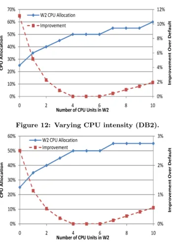
In this set of experiments, we verify that our advisor can accurately respond to the different resource needs of differ-ent workloads. For this experimdiffer-ent, we examine the behav-ior of the 22 TPC-H queries for a database with scale factor 1, and we determine thatQ18 is one of the most CPU inten-sive queries in the benchmark (i.e., its performance improves significantly if it is given more CPU), while Q21 is one of the least CPU intensive queries in the benchmark (i.e., its performance does not improve too much if it is given more CPU). Thus, we use workloads consisting of multiple copies of Q18 and Q21, and we vary the resource needs of the workloads by varying the number of copies of the two query types. One subtle point to note here is thatQ21 has much longer estimated and actual run times thanQ18, so a
vir-Figure 12: Varying CPU intensity (DB2).
Figure 13: Varying CPU intensity (PostgreSQL).
tual machine that is running one copy of Q18 will appear to be “less loaded” than a virtual machine that is running one copy ofQ21, and hence theQ21 VM will be given more resources by our advisor. This would be the correct decision in this case, but we want to make sure that any variation in the resource allocation to the different workloads is due to variations in their resource needs not simply due to having different lengths. Thus, we use 25 copies ofQ18 as our CPU intensive workload “unit”, which we refer to as C, and 1 copy ofQ21 as our CPU non-intensive workload unit, which we refer to as I. To create workloads with different CPU needs, we combine different numbers ofCandIunits. Note that both C andI are decision support queries that both have fairly high CPU demands, even though the demands ofCare greater thanI. Hence, usingCandIfor our work-loads leaves almost no slack for the advisor to improve per-formance. Our purpose in this section is to illustrate that the advisor can detect the different resource needs of the different workloads and improve performance even in this competitive environment.
In our first experiment, we use two workloads that run in two different virtual machines. The first workload consists of 5Cunits and 5Iunits (i.e.,W1= 5C+ 5I). The second
workload hask Cunits and (10−k)I units fork= 0 to 10 (i.e., W2 =kC+ (10−k)I). As k increases, W2 becomes
more CPU intensive whileW1remains unchanged. The
rel-ative sizes of the workloads remain unchanged due to the way we scale C and I to have the same size. Figures 12 and 13 show for DB2 and PostgreSQL, respectively, for
dif-Figure 14: Varying workload size and resource in-tensity (DB2).
Figure 15: Varying workload size and resource in-tensity (PostgreSQL).
ferent values ofk, the amount of CPU allocated toW2 by
our virtualization design advisor (on the lefty-axis) and the estimated performance improvement of this allocation over the default allocation of 50% CPU to each workload (on the righty-axis). For smallk, our design advisor gives most of the CPU toW1 becauseW1 is more CPU intensive. As k
increases, our advisor is able to detect thatW2is becoming
more CPU intensive and therefore it gives W2 more CPU.
Overall performance is improved over the default allocation except in the cases where the two workloads are similar to each other so that the default allocation is optimal. The magnitude of the performance improvement is small because both workloads are fairly CPU intensive so the performance degradation ofW1 when more of the CPU is given toW2 is
only slightly offset by the performance improvement inW2.
The main point of this experiment is that the advisor is able to detect the different resource needs of different workloads and make the appropriate resource allocation decisions.
In our second experiment, we use two workloads that run in two different virtual machines. The first workload con-sists of 1Cunit (i.e.,W3 = 1C). The second workload hask
Cunits fork= 1 to 10 (i.e.,W4=kC). Askincreases,W4
becomes longer compared toW3, and hence more resource
intensive. The correct behavior in this case is to allocate more resources to W4. Figures 14 and 15 show for DB2
and PostgreSQL, respectively, the CPU allocated by our design advisor to W4 for different k and the performance
Figure 16: Varying workload size but not resource intensity (DB2).
Figure 17: Varying workload size but not resource intensity (PostgreSQL).
improvement due to this allocation. Initially, when k= 1, both workloads are the same so they both get 50% of the resources. However, as k increases and W4 becomes more
resource intensive, our search algorithm is able to detect that and allocate more resources to this workload, resulting in an overall performance improvement. The performance improvements in this figure are greater than those in the previous experiment since there is more opportunity due to the larger difference in the resource demands of the two workloads.
Our next experiment demonstrates that simply relying on the relative sizes of the workloads to make resource allo-cation decisions can result in poor decisions. For this ex-periment, we use one workload consisting of 1C unit (i.e.,
W5= 1C) and one workload consisting ofk Iunits fork= 1
to 10 (i.e.,W6=kI). Here the goal is to illustrate that even
thoughW6may have a longer running time, the fact that it
is not CPU intensive should lead our algorithm to conclude that giving it more CPU will not reduce the overall execu-tion time. Therefore, the correct decision would be to keep more CPU with W5 even asW6 grows. Figures 16 and 17
show for DB2 and PostgreSQL, respectively, that our search algorithm does indeed give a lot less CPU toW6than is
war-ranted by its length. W6 has to be several times as long as
W5 to get the same CPU allocation.
It is clear from these experiments that our virtualization design advisor behaves as expected, which validates our
op-Figure 18: Effect of Li.
timizer calibration process and our search algorithm. It is also clear that the advisor is equally effective for both DB2 and PostgreSQL, although the magnitudes of the improve-ments are higher for DB2.
6.4
Supporting QoS Metrics
In this section, we demonstrate the ability of our virtu-alization design advisor to make recommendations that are constrained in accordance with user defined QoS parame-ters (the degradation limit,Li, and the benefit gain factor,
Gi). For this experiment we use five identical workloads,
W7–W11, each consisting of 1 unit of theC workload used
in Section 6.3. The optimal allocation decision in this case is to split the resources equally between the workloads, but we set service degradation limits for two of the workloads to in-fluence this decision. We vary the service degradation limit ofW7,L7, from 1 to 4, and we giveW8 a fixed degradation
limitL8= 2.5.
Figure 18 shows the service degradation of all workloads for different values ofL7. We can see that our virtualization
design advisor is able to meet the constraints specified by
L7 and L8 and limit the degradation thatW7 andW8
suf-fer. This comes at the cost of a higher degradation for the other workloads, but that is expected since theLi
parame-ters specify goals that are specific to particular workloads. We also verified the ability of our advisor to increase the CPU allocation to workloads whose Gi is greater than 1.
We omit the details due to lack of space.
6.5
Random Workloads
The experiments in the previous sections are fairly “con-trolled” in the sense that we know what to expect from the design advisor. In this section, we demonstrate the effective-ness of our advisor on random workloads for which we do not have prior expectations about what the final configura-tion should be. Our goal is to show that for these cases, the advisor will recommend resource allocations that are better than the default allocation.
Each experiment in this section uses 10 workloads. We run each workload in a separate virtual machine, and we vary the number of concurrently running workloads from 2 to 10. For each set of concurrent workloads, we run our design advisor and determine the CPU allocation to each virtual machine and the performance improvement over the default allocation of 1/N CPU share for each workload.
We present results for two random workload experiments.
Figure 19: CPU allocation forN workloads on TPC-H database.
Figure 20: CPU allocation for N OLTP + TPC-H
workloads.
Figure 21: Performance improvement for N
The first experiment uses queries on a TPC-H database with scale factor 10 stored in PostgreSQL. Using a database with scale factor 10 allows us to test our design advisor with long-running resource-intensive queries. For this ex-periment, each of the 10 workloads consists of a random mix of between 10 and 20 workload units. A workload unit can be either 1 copy of TPC-H queryQ17 or 66 copies of a modified version of TPC-HQ18. We added a WHERE pred-icate to the sub-query that is part of the originalQ18 so that the query touches less data, and therefore spends less time waiting for I/O. The number of copies of the modifiedQ18 in a workload unit is chosen so that the two workload units have the same completion time when running with 100% of the available CPU.
The second random workload experiments uses 10 work-loads running on DB2 in different virtual machines. Of these workloads, 5 are OLTP workloads that touch x = 200 to
x= 6000 rows of the table in the OLTP database (W2, W4, W6, W8, and W10). The other 5 workloads consist of up to 40 randomly chosen TPC-H queries.
Figures 19 and 20 show, for both of these experiments, the changes in CPU allocation to the different workloads as we introduce new workloads to the mix. It can be seen that our virtualization design advisor is identifying the nature of new workloads as they are introduced and is adjusting the resource allocations accordingly. The slopes of the dif-ferent CPU allocation lines are not constant. It can also be seen that the advisor maintains the relative order of the workloads’ CPU allocations even as new workloads are in-troduced. The fact that some workload is more resource intensive than another does not change due to the introduc-tion of more workloads.
Figure 21 shows the actual performance improvement un-der different resource allocations for the experiment on the scale factor 10 TPC-H database. The figure shows the per-formance improvement under the resource allocation recom-mended by the virtualization design advisor, and under the optimal resource allocation obtained by exhaustively enu-merating all feasible allocations and measuring performance in each one. The figure shows that our virtualization design advisor, using a properly calibrated query optimizer and a well-tuned database, can achieve near-optimal resource al-locations.
6.6
Online Refinement
In some cases, the query optimizer cost model is inac-curate so our resource allocation decisions are suboptimal and the actual performance improvement we obtain is sig-nificantly less than the estimated improvement. Most work on automatic physical database design ignores optimizer er-rors even if they result in suboptimal decisions. One of the unique features of our work is that we try to correct for op-timizer errors through our online refinement process. In this section, we illustrate the effectiveness of this process using the OLTP + TPC-H workloads from the previous section. Since we are only allocating CPU to the different virtual machines, and since CPU is a resource for which a linear cost model is typically accurate, we use the basic online re-finement approach that is described in Section 5.1.
We expect the query optimizer to be less accurate in mod-eling OLTP workloads than DSS workloads such as TPC-H. The optimizer cost model does not capture contention or up-date costs, which are significant factors in OLTP workloads.
Figure 22: CPU allocation for N OLTP + TPC-H
workloads after online refinement.
Figure 23: Performance improvement for N OLTP
+ TPC-H workloads before and after online refine-ment.
Thus, for our OLTP workload, the optimizer tends to un-derestimate the CPU requirements. The OLTP workload is indeed less CPU intensive than the workloads from TPC-H since I/O is a much higher fraction of its work, but the query optimizer sees it as much less CPU intensive than it really is. It, therefore, leads the advisor to allocate a large portion of the CPU to the workloads from TPC-H. Implementing the CPU allocations recommended by the advisor results in ac-tual performance improvements that are shown in Figure 23. These recommendations are clearly inaccurate. However, if we run our online refinement process on the different sets of workloads, the process converges in at most two iterations and gives the CPU allocations shown in Figure 22. We have verified that these CPU allocations are the same as the opti-mal allocations obtained by performing an exhaustive search that finds the allocation with the lowest actual completion time. In these CPU allocations, the workloads from TPC-H are getting less CPU than before, even though they are longer and more resource intensive. The CPU taken from these workloads is given to the OLTP workloads and pro-vides them with an adequate level of CPU. The resulting actual performance improvements are much better than the improvements without online refinement, and are also shown in Figure 23. Thus, we are able to show that our advisor can provide effective recommendations for different kinds of workloads, giving us easy performance gains of up to 25%.
7.
CONCLUSIONS
In this paper, we considered the problem of automatically configuring multiple virtual machines that are all running database systems and sharing a pool of physical resources. Our approach to solving this problem is implemented as a virtualization design advisor that takes information about the different database workloads and uses this information to determine how to split the available physical computing resources among the virtual machines. The advisor relies on the cost models of the database system query optimizers to enable it to predict workload performance under differ-ent resource allocations. We described how to calibrate and extend these cost models so that they are used for this pur-pose. We also presented an approach that uses actual per-formance measurements to refine the cost models used for recommendation. This provides a means of correcting cost model inaccuracies. We conducted an extensive empirical evaluation of the virtualization design advisor, demonstrat-ing its accuracy and effectiveness.
8.
REFERENCES
[1] R. Agrawal, S. Chaudhuri, A. Das, and V. R.
Narasayya. Automating layout of relational databases. InProc. Int. Conf. on Data Engineering (ICDE), 2003.
[2] P. T. Barham, B. Dragovic, K. Fraser, S. Hand, T. L. Harris, A. Ho, R. Neugebauer, I. Pratt, and
A. Warfield. Xen and the art of virtualization. In
Proc. ACM Symposium on Operating Systems Principles (SOSP), 2003.
[3] M. Bennani and D. A. Menasce. Resource allocation for autonomic data centers using analytic performance models. InProc. IEEE Int. Conf. on Autonomic Computing (ICAC), 2005.
[4] M. J. Carey, R. Jauhari, and M. Livny. Priority in DBMS resource scheduling. InProc. Int. Conf. on Very Large Data Bases (VLDB), 1989.
[5] D. L. Davison and G. Graefe. Dynamic resource brokering for multi-user query execution. InProc. ACM SIGMOD Int. Conf. on Management of Data, 1995.
[6] K. Dias, M. Ramacher, U. Shaft, V. Venkataramani, and G. Wood. Automatic performance diagnosis and tuning in Oracle. InProc. Conf. on Innovative Data Systems Research (CIDR), 2005.
[7] M. N. Garofalakis and Y. E. Ioannidis.
Multi-dimensional resource scheduling for parallel queries. InProc. ACM SIGMOD Int. Conf. on Management of Data, 1996.
[8] A. Karve, T. Kimbrel, G. Pacifici, M. Spreitzer, M. Steinder, M. Sviridenko, and A. Tantawi. Dynamic placement for clustered web applications. InProc. Int. Conf. on WWW, 2006.
[9] G. Khanna, K. Beaty, G. Kar, and A. Kochut. Application performance management in virtualized server environments. InProc. IEEE/IFIP Network Operations and Management Symp. (NOMS), 2006. [10] P. Martin, H.-Y. Li, M. Zheng, K. Romanufa, and
W. Powley. Dynamic reconfiguration algorithm: Dynamically tuning multiple buffer pools. InProc. Int. Conf. Database and Expert Systems Applications (DEXA), 2000.
[11] M. Mehta and D. J. DeWitt. Dynamic memory allocation for multiple-query workloads. InProc. Int. Conf. on Very Large Data Bases (VLDB), 1993. [12] D. Narayanan, E. Thereska, and A. Ailamaki.
Continuous resource monitoring for self-predicting DBMS. InProc. IEEE Int. Symp. on Modeling, Analysis, and Simulation of Computer and Telecommunication Systems (MASCOTS), 2005. [13] OSDL Database Test Suite 3.
http://sourceforge.net/projects/osdldbt.
[14] M. Rosenblum and T. Garfinkel. Virtual machine monitors: Current technology and future trends.IEEE Computer, 38(5), 2005.
[15] P. Ruth, J. Rhee, D. Xu, R. Kennell, and
S. Goasguen. Autonomic live adaptation of virtual computational environments in a multi-domain infrastructure. InProc. IEEE Int. Conf. on Autonomic Computing (ICAC), 2006.
[16] P. Shivam, A. Demberel, P. Gunda, D. E. Irwin, L. E. Grit, A. R. Yumerefendi, S. Babu, and J. S. Chase. Automated and on-demand provisioning of virtual machines for database applications. InProc. ACM SIGMOD Int. Conf. on Management of Data, 2007. Demonstration.
[17] J. E. Smith and R. Nair. The architecture of virtual machines.IEEE Computer, 38(5), 2005.
[18] A. A. Soror, A. Aboulnaga, and K. Salem. Database virtualization: A new frontier for database tuning and physical design. InProc. Workshop on Self-Managing Database Systems (SMDB), 2007.
[19] M. Steinder, I. Whalley, D. Carrera, and I. G. D. M. Chess. Server virtualization in autonomic management of heterogeneous workloads. InProc. IFIP/IEEE Int. Symp. on Integrated Network Mgmt., 2007.
[20] A. J. Storm, C. Garcia-Arellano, S. Lightstone, Y. Diao, and M. Surendra. Adaptive self-tuning memory in DB2. InProc. Int. Conf. on Very Large Data Bases (VLDB), 2006.
[21] C. Tang, M. Steinder, M. Spreitzer, and G. Pacifici. A scalable application placement controller for enterprise data centers. InProc. Int. Conf. on WWW, 2007. [22] G. Tesauro, R. Das, W. E. Walsh, and J. O. Kephart.
Utility-function-driven resource allocation in
autonomic systems. InIEEE Int. Conf. on Autonomic Computing, 2005.
[23] VMware. http://www.vmware.com/. [24] X. Wang, Z. Du, Y. Chen, and S. Li.
Virtualization-based autonomic resource management for multi-tier web applications in shared data center.
Journal of Systems and Software, 2008.
[25] X. Wang, D. Lan, G. Wang, X. Fang, M. Ye, Y. Chen, and Q. Wang. Appliance-based autonomic
provisioning framework for virtualized outsourcing data center. InProc. IEEE Int. Conf. on Autonomic Computing (ICAC), 2007.
[26] G. Weikum, A. M¨onkeberg, C. Hasse, and P. Zabback. Self-tuning database technology and information services: from wishful thinking to viable engineering. InProc. Int. Conf. on Very Large Data Bases (VLDB), 2002.