JEEECCS, Volume 1, Issue 2, pages 15-20, 2015
Evaluation of Parallelism in Ant Colony
Optimization Method for Numerical Solution
of Optimal Control Problems
H.H. Mehne Aerospace Research Institute
Tehran, IRAN [email protected]
Abstract – In this paper, the ant colony optimization (ACO) method for solving optimal control problems is investigated from parallel processing viewpoint. The OpenMP implementation of this method is presented and compared with the MPI implementation. A numerical example is also given to show the accuracy of the method and to evaluate the parallel performance.
Keywords: Optimal control; parallel processing; ant colony optimization; OpenMP
I. INTRODUCTION
The complexity of solving optimal control problem analytically motivates many researchers in different fields of science and engineering to develop numerical methods. Numerical methods for solving optimal control problems are categorized as direct and indirect methods. Indirect methods arisen from optimality conditions known as maximum principle. In such a method, instead of the original problem, the equivalent Hamilton Jacobi problem is solved numerically. Indirect methods are accurate but they have low convergence rate and finding initial guess for adjoint variables is difficult. As a recent reference on indirect methods we may address [1] in which an iterative method for affine nonlinear optimal control problems is proposed.
In direct methods, on the other hand, the optimal control problem is transformed directly to a finite dimensional optimization problem. This may done by discretization of the time domain to multi stages or by direct collocation,where the state or control variable is parameterized. Larger domain of convergence is advantage of these methods, while they have low accuracy with respect to indirect ones. Different viewpoints of transformation in direct methods alongside with different optimization methods lead to various numerical algorithms with different of theoretical basis, accuracy and convergence rate. In [2] for example, parameterization of state variable is used. In [3] measure theory method is applied to drive a linear programming framework. Ant colony optimization method (ACO) is used in [4] to solve the corresponding nonlinear programming problem that arises from time domain multi staging. This method is more investigated and developed in [5,6]. One of the ant colony method's profits is its parallelization nature. According to this fact, the method of [4] is then
implemented parallel using MPI library in [7]. By this modification, one can benefit from parallel processing aspects in solving larger problems faster than serial case.
The aim of this article is to change the method of [7] to adopt with OpenMP approach which is another parallel programming style fitting multiprocessor /multicore computers. Then, the proposed approach will be compared with MPI application of the ant colony method for optimal control problems. Implementation, parallel performance and accuracy are explained on a case study.
II. DESCRIPTION OF THE PROBLEM
There are many problems in economics, aeronautics, robotics, space vehicle and satellite control which are formulated as optimal control governing by a system of ordinary dynamical system like:
̇ ( ) (1) The aim of these problems is to determine input vector ( ) in such a way that a combination of the control and related response of (1) as a performance index like the following be minimized or maximized:
∫ ( ( ) ( )) (2)
There is also a given initial point in the state space, for example, ( ) .
A. Multiple-stepping
The described problem has a discretized or multiple-step form obtained by dividing the time interval , - into subintervals or steps as follows:
, - , - , - (3)
Where, and . Assume that and denote respectively the control and related state at . Then, the original problem is converted to a nonlinear programming problem as minimization of
∑ ( ̅ )
(4)
( ̅ ) (5) According to the method of integration, ̅ stands for a vector of and its predecessors. If Euler or Runge-Kutta method is used, then ̅ includes only . Starting with , and using an optimization procedure, one can solve the problem numerically. If we are satisfied only with grid point values of and
, then,these values will be found by solving the above problem. In the method of [8], for example, the discrete form is reduced to a linear programming problem. However, when more accurate solution is required, integration between steps is needed which is called multi-staging, an example is iterative dynamical programming method [9].
Discussed in the next section, the ACO method for solving optimal control problems which has been proposed in [4] is based also on (4)-(5) formulation with multi staging.
III. THE ACOMETHOD
In the ACO solution of optimization problems, as in the optimization problem (4)-(5), it is assumed that the control function is constant on each stage , -and its value is shown with . The values are output of dividing the set of prescribed control interval. Assume that the allowable control values is
, - and is divided to point as * +. Now, any piecewise constant function like
( ) ∑ (, -)
( ) (6)
is an admissible control function in piecewise constant form, where is any permutation of
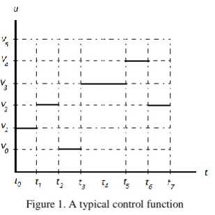
* +and ( ) is the characteristic function. Indeed, in the divided time-control space, there is a grid, and a control function of the form of (6) is a step function in this grid. Such a control function is shown in Fig.1. In this example, , and so on.
It is clear that, any combination of s in (6) leads to a solution of the problem with different objective function. In the ACO method, the task of examining of this different paths in time – control space is done by some agents called ants. There are a defined number of
ants that taking tours on this space and then evaluate the vector from (5) and corresponding performance index from (4). Then, each ant returns its evaluation and then, an optimum path will result among different tries of these agents.
According to the optimum solution, the ants trace on the time – control space will be updated. The method iterates until a convergence occurs. Below, the method is described.
A. The serial version
The steps of the main ACO for optimal control problems are as follows ([7]):
Initialization: In this step, initial values of
pheromone trails are set. For starting, the values of pheromone corresponding to the
assignment of to for -th ant are set to 1.
Probabilities Calculation: After calculating of
pheromones, the values of probabilities are calculated by:
∑
(7)
which determines the probability for -th ant to choose for -th subinterval.
Path Construction: The above probabilities
determine one path in the time-control space or equivalently a control function.
Index Evaluation: In this step, the
corresponding initial value problem with control function as input is solved by Runge-Kutta method. Then, a numerical estimation for the performance index is calculated for each ant. This value is a measure to estimate the fineness of the resulting control function.
Finding the Best Solution: After calculating
performance indices for all ants, we will find the optimum solution among all ants’ results. This is referred by global optimum.
Updating Pheromone Trails: First we should
decrease the pheromones by an evaporation to avoid unlimited accumulation of pheromone trails. This is done by setting
( ) (8)
for all , , . In the above equation, is the constant evaporation rate. Then, we should increase the pheromone trails in all solution if the corresponding time-control is also in the optimum solution. This will do as:
∑
(9)
where, is equal to the inverse of global optimum if ( ) in the current optimal solution and in the solution of ant with optimum performance index. As the default value for is zero, by this method we increase the probability of choosing good time-control assignments in the next iterations.
The process will return to the step of probability construction if we don’t reach to the end of iterations. The flowchart of serial ACO algorithm for solvingthe present problem is depicted in Fig.2.
There are many references on evaluating the computational complexity of the original ACO algorithm (see [10], for example). Here, we discuss the complexity computation of the version for optimal control problems.
With a fixed number of iterations, the upper bound of the computational complexity of the sequential method is ( ), where, and
stand for number of iterations and number of ants, respectively. Indeed, the computational complexity of one iteration of the algorithm with one ant is of order ( ) .
B. Parallel Version: MPI
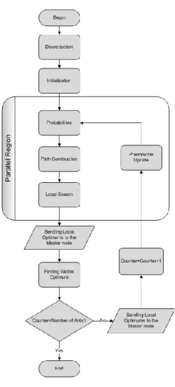
As the tasks assigned to each ant are independent to the tasks of the others, this section including probabilities construction, path construction, finding minimum and pheromone update may fulfill in parallel. The parallel version is presented and analyzed in [7] with using MPI library implementation. The related flowchart is depicted in Fig.3.
There are here two communication points in each iteration. Via a local search, each ant calculates a local optimum, and then, they send the master node their local optimums. The master node finds the global optimum and then sends the updating pheromone information back to the workers. As reported in [7], on a test case with 16 processors, the parallel efficiency reaches to 87%. The MPI approach may applied to both distributed and shared memory hardware, but the above mentioned data connection affects the performance, especially for large-scale problems and for large number of processors.
In the MPI parallelism, the serial part of the program has ( ) ( ) computational complexity, and the parallel part has
( ) complexity which is divided between processors. Moreover, there is communication time for send-receive and for
Begin
Discretization
Initialization
Pheromone Update
End Counter<Number of Ants?
Yes Probabilities
Path Construction
Find Optimum
No Counter=Counter+1
broadcast which totally is of order ( ). Therefore, the overall computational complexity upper bound is:
. / ( ).
The above relation shows that the impact of the communication on the overall complexity. If , then the computation cost dominates the communication. But for the problems with low size, the effect of the communications will show itself by decreasing the speed up and related performance.
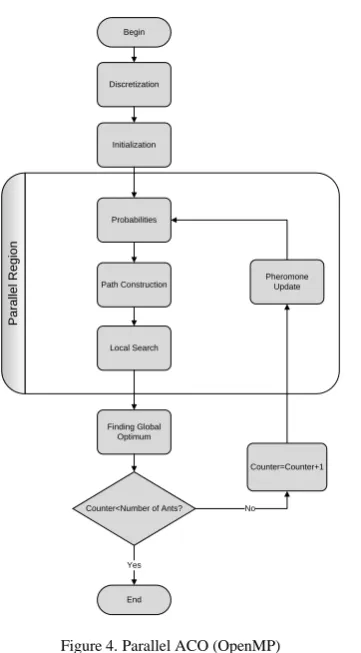
C. Parallel Version: OpenMP
OpenMPI is an application programming interface for parallel processing on shared memory architectures. It uses a portable, scalable model that gives programmer a simple and flexible interface. The main program is divided to serial and parallel regions. When the processors enter the parallel region of the algorithm, they run instructions as individual threads.
When OpenMP is used to ACO method for solving optimal control problems, then the phase of sending local optimums to the master node and giving back the update information is not required. In the OpenMP programming, data will be captured from shared location in the memory. This reduces the cost of communication with respect to MPI implementation.
Fig. 4 shows the flowchart of the OpenMP implementation of the method.
When OpenMP parallelization is used, computations is divided vi threads. Suppose that the
number of processors is . Then complexity of serial part of the program is ( ) ( ) for discretization and finding optimum functions. The parallel part has also ( ) complexity which is divided through threads. Therefore, the total upper bound of the computational complexity in the case of OpenMP implementation equals ( )which is times less than the sequential case. Moreover, comparing this result with complexity of MPI method shows more expected performance for OpenMP. Consider one ant one iteration of MPI and OpenMP method. The corresponding complexities are respectively
. ⁄ / ( ), and ( ). So, for larger than , the OpenMP method has better performance. It is also to be mentioned that with MPI, the performance decrease with increasing , as in the numerical example of [7], when is increase after 10, then the seed up curve starts diverging from ideal condition. This is because of growing with constant in
. ⁄ / ( ), which causes the domination of communication term ( ) to the computation one.
IV. NUMERICAL EXAMPLE
In order to examine the method, a benchmark nonlinear control problem from [11] is used. The problem is called low thrust rendezvous which deals with planer relative motion of two particles in a central gravity field expressed in a rotating frame with normalized units. The state vector ( ) contains radial and tangential displacements and velocities. The control vector ( ) consists of radial and tangential accelerations. The dynamic of this problem in which the rotational and translational motion of an actuator are coupled is as follows:
̇ ̇
̇ ( ) ( )
̇ ( )
where √( ) . Initial conditions are also given as:
( ) ( ) ( ) ( )
The object of the soft constrained rendezvous problem is to find the control functions ( )
, - , ( ) , - that minimize the missed distance and implemented thrusts. This is formulated as the following performance index:
( ) ( ) ∫ ( )
where, and ( ) is a weight vector forcing the final conditions to be zero.
We solved the above problem with the proposed method on Aerospace Research Institute's parallel
Begin
Discretization
Initialization
Pheromone Update
End Counter<Number of Ants?
Yes Probabilities
Path Construction
Local Search
Finding Global Optimum
No
Counter=Counter+1
P
a
ra
lle
l
R
e
g
io
n
processing system having 32 AMD processors with 2.8GHz clock speed.The system has an Infiniband network with 10 GB/s bandwidth and 0.7 microsecond latency.
The program has been developed with C++ language and was compiled with gcc-4.3.4 with integrated OpenMP. For MPI library, the OpenMPI 2.0 was used.
Parameters of this numerical simulation are shown in Table.1.
TABLE I. PARAMETERS
AntNo IterNo.
80 35 0.065 30 5 5
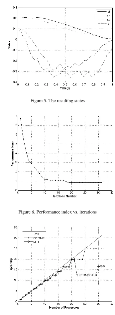
The resulting state vectors are given in Fig.5. The missed distance vector is (0.004, 0.024, -0.002, -0.063) which has an acceptable accuracy.
The rate of convergence is also presented in Fig.6, where the performance index is drawn in terms of iteration number. It shows that the performance index decreases in each iteration until converges with an exponential rate to .
In order to compare the performance of the proposed method with the method of [7], the problem with the same parameters has been also solved with the MPI method. The corresponding speed up graphs are compared in Fig.7. It is clear that up to 20 processors, the two speed up curves coincide each other and with the ideal line. By increasing the number of processors, as expected, the MPI speed up diverges from its trend while the OpenMP speed up keeps its increasing behavior. Results for this case with 32 processors show that, the maximum speed up for OpenMP is 24 and for MPI is 16. Therefore, OpenMP implementation leads to 50% more speed up and 15% increment in parallel performance.
Indeed, as stated in part B of section III, the overcome of communication to computation after 20 processors causes the reduction in the speed up.
V. CONCLUSIONS
The OpenMP parallelization of the ant colony optimization method for numerical solution of optimal control problems is presented. Complexity analytical of serial and two parallel approach is also given. A numerical example is used to check the accuracy of the method and to compare parallel performance of these two approaches. Results show that with increasing the number of processors, the OpenMP approach has better performance than the MPI, while it is restricted to special computer architecture with multiprocessors. The MPI method, on the other hand, can be implemented on both shared and distributed architectures, while its speed up is reduced with respect to OpenMP because of more data communications.
For further development of the ACO method for optimal control problems, extension of the method to GPU programming is suggested.
REFERENCES
[1] B. Luo, H-N, Wu, T. Huang, and D. Liu, “Data-based approximate policy iteration for affine nonlinearcontinuous-time optimal control design,” Automatica, vol. 50, pp. 3281– 3290, 2015.
[2] H.H. Mehne, and A.H. Borzabadi, “A numerical method for solving optimal control problems using state Figure 5. The resulting states
Figure 6. Performance index vs. iterations
parametrization”, Numerical Algorithms, vol. 42, no. 2, pp. 165–169, 2006.
[3] H.H. Mehne, M.H. Farahi, and A.V. Kamyad, “MILP modelling for the time optimal control problem in the case of multiple targets”, Optimal Control Applications and Methods, 27:77–91, 2006.
[4] A. Borzabadi, and H. Mehne, “Ant colony optimizationfor optimal control problems”, Journal of Information and Computing Science, 4(4):259–263, 2009.
[5] A. Borzabadi, M. Heidari, “Evolutionary Algorithms for Approximate Optimal Control of the Heat Equation with Thermal Sources ”, Journal of Mathematical Modelling and Algorithms, vol.11, no.1, pp. 77-88, 2012.
[6] A. P. Pourhashemi, and S. M. Mehdi Ansarey M., “Ant Colony Optimization Applied to Optimal Energy Management of Fuel Cell Hybrid Electric Vehicle”,
4thInternational Congress on Ultra Modern
Telecommunications and Control Systems and Workshops, 2012
[7] H.H. Mehne, A. Aliparast, “A Parallel Numerical Method for Solving Optimal Control Problems”, ICTPE 2015, pp.252-256, 2015.
[8] H.H. Mehne, “A numerical method for solving linear time-varying systems based on linear programming”, Applied Mathematics and Computation, vol. 178, pp. 287-294, 2006. [9] R. Luss, “Iterative Dynamic Programming”, Chapman &
Hall, CRC, 2000.
[10] F. Neumann, D. Sudholt, C. Witt, “Computational complexity of ant colony optimization and its hybridization with local search”, Innovations in Swarm Intelligence, pp. 91-120, Springer, 2009.