Available online throug
ISSN 2229 – 5046
EOQ MODEL WITH SHORTAGES IN BEGINNING
AND PERIODIC DEMAND FOR DETERIORATING ITEMS
UTTAM KUMAR KHEDLEKAR*
Department of Mathematics and Statistics,
Dr. Harisingh Gour Vishwavidyalaya Sagar, Madhya Pradesh, India, 470003.
(A Central University)
(Received On: 28-10-15; Revised & Accepted On: 18-11-15)
ABSTRACT
M
any products exists in nature which follows repetitions of demand pattern. For example, demand of water cooler is high in summer and low in winter and again increases as temperature increases and hence the demand pattern is periodic. So, we need to develop a new inventory model for such kind of products. In this paper an economic order quantity model has been presented for deteriorating item with periodic demand. Also one can start business with shortage like advance booking of products which could be fulfilled after time duration. We have incorporated the shortage at the beginning of the sale season. A new model is developed and optimal shortage duration is obtained along-with some other results. Simulation study is performed along with managerial insights. Proposed model is found useful for products having periodic demand pattern and bearing shortage at the starting.Keywords: Inventory, Periodic Demand, Deterioration, Shortage, Replenishment time.
1. INTRODUCTION
In past, Harris (1915) and many researchers have been suggested inventory models with variety of demand functions. There are many products that follow periodic demand pattern and need to develop new inventory model. Also a business could be started with shortage like advance booking of LPG gas, electricity supply and pre public offer of equity share before proper functioning of a company. We incorporate two features: one is periodic demand and other is start of business with shortage in the proposed model. Few items in the market are of high need for people like sugar, wheat, oil whose shortage break the customer’s faith and arrival pattern. This motivates retailers to order for excess units of item for inventory in spite of being deteriorated. Moreover, deterioration is manageable for many items by virtue of modern advanced storage technologies. Inventory model presents a real life problem (situation) which helps to run the business smoothly. Our aim is to solve the problem of the business which start with shortage and in which the demand of the products follow the periodic demand.
Burwell et al. (1997) solved the problem arising in business by providing freight discounts and presented an economic lot size model with price-dependent demand. Shin (1997) determined an optimal policy for retail price and lot size under day-term supplier credit policies based on constant demand where after maturing the product in market, it follows linear demand.
Matsuyama (2001) presented a general EOQ model considering holding costs, unit purchase costs, and setup costs that are time-dependent and continuous general demand functions. The problem has been solved by dynamic programming so as to find ordering point, ordering quantity, and incurred costs. A research overview by Emagharby and Keskinocak (2003) is for determining the dynamic pricing and order level. Teng and Chang (2005) presented an economic production quantity (EPQ) model for deteriorating items when the demand rate depends not only on the on-display stock, but also on the selling price per unit considering market demand. The manipulation in selling price is the best policy for the organization as well as for the customers. Wen and Chen (2005) suggested a dynamic pricing policy for selling a given stock of identical perishable products over a finite time horizon on the internet. The sale ends either when the entire stock is sold out, or when the deadline is over. Here, the objective of the seller is to find a dynamic pricing policy that maximizes the total expected revenues. Shukla and Khedlekar (2009) introduced the concept of three warehouses in which one oriented and two rented warehouses to store the deteriorating items as per requirements.
The EOQ model designed by Hou and Lin (2006) reflects how a demand pattern which is price, time, and stock dependent affects the discount in cash. They discussed an EOQ inventory model which takes into account the inflation and time value of money of the stock-dependent selling price. Existence and uniqueness of the optimal solution has not been shown in this article. Lai et al. (2006) algebraically approached the optimal value of cost function rather than the traditional calculus method and modified the EPQ model earlier presented due to Chang (2004) in which he considered variable lead time with shortage. Chandel and Khedlekar (2013) also used multiple warehouses on location based and ordered quantity as centralised basis and minimized the incurred cost. Recent contribution in EPQ models is a source of esteem importance like Birbil et al. (2007), Hou (2007), Khedlekar and Shukla (2015), Bhaskaran et al. (2010), Jogelekar et al. (2008), Roy (2008), Kumar (2012a, b, c) and You (2005). Motivation is derived due to Wu (2002) and Shukla et al. (2010, 2014), Khedlekar et al. (2013) for considering the shortages in beginning of a business and henceforth developed the proposed model. Section 2 consists of the assumption and notations of the model while a section 3 deal with the mathematical formulation of model, section 4 is for numerical example and simulation.
2. ASSUMPTIONS AND NOTATIONS
Suppose demand of a product is asin(bt). In starting supposeshortage accumulated till time t1 so that on hand shortage is I1(t).The order receives to the company by vendor at t1 and so the shortage ends and inventory reaches up to level I2(t1). This inventory level is sufficient to fulfil the demand till time T. Our aim is to find the optimal time t1 to optimize the total inventory cost. Inventory depleted due to demand and deterioration as shown in fig 1.
The followings notations are used to develop the proposed model.
D(t) demand of product is
D
(
t
)
=
a
sin(
bt
)
where a and b >1 are positive real values.θ rate of deterioration of product, θ <1. c1 holding cost unit per unit time. c2 shortage cost unit per unit time. c3 deterioration cost.
T cycle time. *
1
t optimal time for accumulated shortages. I1(t) on hand shortage of the product (I1(t) > 0). I2(t) on hand inventory of the product (I2(t) > 0). C(t1) optimal inventory cost.
DT deteriorated units.
ST shortage units in the system. SC shortage cost.
HC holding cost. DC deterioration cost.
3. MATHEMATICAL MODEL
Suppose on hand shortage is by I1(t) and this accumulates until t1. Management has placed the order which fulfilled at time t1 and thus on hand inventory is I2(t1).After time t1, theinventory depleted due to demand and deterioration then it reduces to zero at time T (see Fig. 1).
)
sin(
)
(
1
t
a
bt
I
dt
d
=
−
, where 0≤ ≤t t1, I1(0) 0= (1)
)
sin(
)
(
)
(
22
t
I
t
a
bt
I
dt
d
+
θ
=
−
, where
t
1≤
t
≤
T
(2)Boundary conditions for above two differential equations areI1(0)=0, I T2( ) 0,= solving equation (1) we get
(
1
cos(
)
)
)
(
1bt
b
a
t
I
=
−
(3)Solving equation (2) we get
(
sin(
)
cos(
)
)
(
sin(
)
cos(
)
)
)
(
2 2 2 22
e
bt
b
bt
b
a
a
bT
b
bT
e
b
a
a
t
I
T t t+
+
−
+
+
=
θ −θθ
−θθ
(4)
Deteriorated units in time
(
t
1,
T
]
isD
T∫
−
=
Tt
T
I
t
a
bt
D
1)
sin(
)
(
1 2
−
=
b
bt
t
b
ac
1 12
sin(
(5)Holding cost HC over time
(
t
1,
T
]
will be(
)
(
)
(
)
2 2 1 1 2 2sin(
)
cos(
)
sin(
)
sin(
)
cos(
)
cos(
)
t T
T
t
a
e
e
e
a
bT
b
bT
a
b
HC
h
a
b
bT
b
bt
bT
bt
b a
b
θ θ θ
θ
θ
θ
− −
−
+
+
=
−
−
−
+
+
(6)Shortages 1
(
1)
(
1
cos(
bt
1)
)
b
a
t
I
=
−
(
1
cos(
1)
)
2
bt
b
ac
S
C=
−
(7)Number of units including shortage in business schedule is
)
(
)
(
1 2 1 1t
I
t
I
Q
=
+
(8)Total average inventory cost will be
+ + = T D S H t
C(1) C C C
(9)
(
)
(
)
−
+
+
+
−
=
− −θ
θ θθT
e
te
TbT
b
bT
a
e
b
a
a
h
bt
b
ac
T
1
cos(
)
sin(
)
cos(
)
1
2 2 1 1 2(
)
(
)
+
−
−
+
−
−
+
1 2 1sin(
1 2 2b
sin(
bT
)
b
sin(
bt
)
cos(
bT
)
cos(
bt
1)
b
a
b
a
b
bt
t
b
ac
T
h
t
θ
θ
(10)To optimize the total cost function (C(t1)) first derivative equating to zero
(
)
(
)
+
+
+
+
+
−
=
−)
sin(
)
cos(
)
(
)
cos(
)
sin(
1
)
(
1 21 2 2 1 2 2 1 11
1
b
bt
b
bt
b
a
b
ah
e
bT
b
bT
a
b
a
e
ah
T
t
C
dt
d
θT θtθ
(
)
(
)
1 2 3 3 1 12 2 2 2
1 1
sin( ) cos( ) cos( ) sin( )
T t
ac e ac
a bT b bT n bt b bt
T a b T a b
θ θ θ − − + − − + +
1 ac3sin(bt1) ac2 ac2cos(bt1)
T b b
+ + −
On equating
(
1)
0
1
=
t
C
dt
d
, we get equation for optimality value of say which is
t
1=
t
1* Condition for optimality is0
)
(
12 1 2
>
t
C
dt
d
(12)
Thus Average total cost is optimum at
t
1=
t
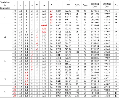
1*.Table-1: Sensitivity of different parameters Variation
in Parameter
a b c1 c2 C3 ө T t1 TC Q(T) I2(t2)
Holding Cost
Shortage Cost DT
T
10 0.2 1 2 2 0.01 14 4.234 122.43 101 51 1378.56 49.34 4 10 0.2 1 2 2 0.01 12 5.108 89.58 95 45 691.700 49.99 2 10 0.2 1 2 2 0.01 10 5.713 68.47 80 30 281.140 1.000 0 10 0.2 1 2 2 0.01 08 6.125 60.11 62 13 70.2400 48.88 0 10 0.2 1 2 2 0.01 07 6.266 61.56 53 5 19.2000 48.59 0
Ө
10 0.2 1 2 2 0.005 14 4.600 120.99 104 55 1338.05 49.82 2
10 0.2 1 2 2 0.01 14 4.234 122.43 101 52 1378.56 49.35 4
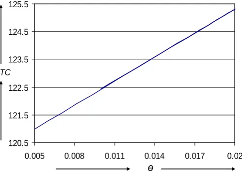
10 0.2 1 2 2 0.02 14 3.406 125.32 76 29 1475.17 47.07 9
10 0.2 1.4 9 3 0.01 14 5.855 243.66 115 66 1574.80 49.35 2 10 0.2 1.4 9 4 0.01 14 5.841 243.96 115 66 1577.92 49.37 2 10 0.2 1.4 9 5 0.01 14 5.826 244.26 115 66 1581.28 49.40 2 10 0.2 1.4 9 6 0.01 14 5.812 244.55 115 66 1584.41 49.42 3 10 0.2 1.4 9 7 0.01 14 5.798 244.85 115 66 1587.54 49.44 3 10 0.2 1.4 9 8 0.01 14 5.781 245.16 115 66 1591.32 49.46 3
c2
10 0.2 1.4 3 2 0.01 14 4.465 171.68 104 54 1880.65 49.68 4 10 0.2 1.4 4 2 0.01 14 5.048 179.63 110 60 1753.92 50.00 3 10 0.2 1.4 5 2 0.01 14 5.361 190.61 113 63 1684.85 49.89 3 10 0.2 1.4 6 2 0.01 14 5.559 202.94 114 64 1640.87 49.73 3 10 0.2 1.4 7 2 0.01 14 5.695 216.02 115 65 1610.55 49.58 3 10 0.2 1.4 8 2 0.01 14 5.794 229.55 115 66 1588.45 49.44 2 10 0.2 1.4 9 2 0.01 14 5.870 243.36 115 66 1571.44 49.33 2
c1
10 0.2 1.5 2 2 0.01 14 2.520 187.58 65 23 2435.09 42.38 5 10 0.2 0.8 2 2 0.01 14 4.740 100.58 107 57 1040.70 49.92 3 10 0.2 0.9 2 2 0.01 14 4.496 111.26 104 55 1204.71 49.71 4 10 0.2 1.2 2 2 0.01 14 3.648 146.45 91 44 1759.14 47.92 4 10 0.2 1.4 2 2 0.01 14 2.957 172.96 77 32 2190.11 45.02 5
A
15 0.2 1.4 2 2 0.01 14 2.957 200.82 115 47 2464.51 67.53 7 20 0.2 1.4 2 2 0.01 14 2.955 228.69 153 63 2739.45 90.03 9 25 0.2 1.4 2 2 0.01 14 2.954 256.56 191 79 3014.24 112.5 11 30 0.2 1.4 2 2 0.01 14 2.953 284.43 230 95 3289.10 135.0 13
4. NUMERICAL EXAMPLE AND SIMULATION
Let us assume that model parameters are a = 10 units, b = 0.2, c1 = $1 per unit per month, c2 = $2 per unit per month, C3 = $2 per unit per month, θ = 0.01, T = 14 days and demand of the product isD t( )=asin(bt).Under the given parameter values and by equation (6) to (10) we get output parameters t1= 4.23days, average total inventory cost TC = $122.43.93, Q = 101 units, average holding cost HC = $98.46.
Now, in this section, we study how the input parameters change significantly to the output parameters. We change the value of one input parameter, keeping other parameters constant. The output parameter is valuated for decision making. The data used for this purpose is in section 4.
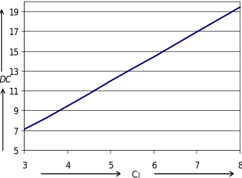
Management needs to be aware about the deterioration cost and holding cost both and tries to keep it as low as possible. High initial demand (parameter a) increases the EOL and EOQ both (table 1), but optimal time interval of these two remain unchanged. From table 1, it is observed that the optimal time is highly sensitive for deterioration and holding cost.
Figure 2. Effect of time cycleon total cost
104 106 108 110 112 114 116
3 4 5 6 7 8 9
Q
c
2Figure 3. Effect of shortage cost on total quantity
5 7 9 11 13 15 17 19
3 4 5 6 7 8
C3 DC
Figure 4. Effect of deterioration ratte on deterioreted cost 59
69 79 89 99 109 119
7 9 11 13
120.5 121.5 122.5 123.5 124.5 125.5
0.005 0.008 0.011 0.014 0.017 0.02
TC
ө
Figure 5. Effect of deterioration rate on total cost
5. CONCLUSIONS
A mathematical inventory model is suggested in the content for a business that starts with shortages and free to place the order according to the demand and customer’s response. Inventory managers should keep the deterioration rate as low as possible because it increases the wastage of quantity as well as the total cost. However one can negotiate the shortage cost to customers, which may keep lower to the incurred cost. Suggested model is sensitive for deterioration and holding cost both as compared to shortage cost for a product having periodic demand. This model can be further extended for variable deterioration, ramp type demand and for finite rate of replenishment. This model may also be formulated in the fuzzy environment.
REFERENCES
1 Bhaskaran S, Ramachandran K and Semple J, A dynamic inventory model with the right of refusal. Management Science, 56 (12) (2010) 2265-2281.
2 Birbil SI, Frenk JBG & Bayindir ZP, A deterministic inventory/production model with general inventory cost rate function and piecewise linear concave production costs. European Journal of Operational Research, 179(1) (2007) 114-123.
3 Burwell T, Dave DS, Fitzpatrick K E & Roy M R, Economic lot size model for price dependent demand under quantity and fright discount. International Journal of Production Economics, 48(2) (1997) 141-155.
4 Chandel RPS & Khedlekar UK, A new inventory model with multiple warehouses. International Research Journal of Pure Algebra Research, 3(5) (2013), 192-200.
5 Chang HC, A note on the EPQ model with shortages and variable lead time. International Journal of Information Management Sciences, 15 (2004) 61-67.
6 Emagharby & Keskinocak P, Dynamic pricing in the presence of inventory considerations: research overview-Current practice and future direction. Management Science, 49(10) (2003) 1287-1309.
7 Harris FW, What quantity to make at once the library of factory management. Operations and Costa (A. W. Shaw Company, Chicago), 5 (1915), 47-52.
8 Hou KL & Lin LC, An EOQ model for deteriorating items with price and stock dependent selling price under inflation and time value of money. International Journal of System Science, 37(15) (2006) 1131-1139.
9 Hou KL, An EPQ model with setup cost and process quality as functions of capital expenditure. Applied Mathematical Modeling, 31(1) (2007) 10-17.
10 Joglekar P, Lee P & Farahani AM, Continuously increasing price in an inventory cycle: An optimal strategy for E-tailors. Journal of Applied Mathematics and Decision Science, 8 (2008) 1-14.
11 Khedlekar UK & Shukla D, Dynamic pricing model with logarithmic demand. Opsearch, 50(1) (2013) 1-13. 12 Khedlekar UK & Shukla D, Simulation of economic production quantity model for deteriorating item,
American Journal of Modeling and Optimization, 1(3) (2013), 25-30.
13 Khedlekar UK, Shukla D & Chandel RPS, Computational study for disrupted production system with time dependent demand. Journal of Scientific and Industrial Research, 73(5)(2014)294-301.
14 Khedlekar UK, Shukla D & Chandel RPS, logarithmic inventory model with shortage for deteriorating items. Yugoslav Journal of Operations Research, 23(3) (2013) 431-440.
16 Kumar R & Sharma SK, Formulation of product replacement policies for perishable inventory systems using queuing theoretic approach. American Journal of operational Research, 2(4) (2012b) 27-30.
17 Kumar, R., and Sharma, S.K., “Product replacement strategies for perishable inventory system using queuing theory”, Journal of Production Research and Management, 2(3) (2012c) 17-26.
18 Lai C S, Huang Y F & Hung H F, The EPQ model with shortages and variable lead time. Journal of Applied Science, 6(4) (2006) 755-756.
19 Matsuyama K, The general EOQ model with increasing demand and costs. Journal of Operations Research, 44(2) (2001) 125-139.
20 Roy A, An inventory model for deteriorating items with price dependent demand and time-varying holding cost. Advanced Modeling and Optimization, 10(1) (2008) 25-37.
21 Shin S W, Determining optimal retail price and lot size under day-term supplier credit. Computers & Industrial Engineering, 33(3) (1997) 717-720.
22 Shukla D & Khedlekar UK, An inventory model with three warehouses. IndianJournal of Mathematics and Mathematical Sciences, 5(1) (2009), 39-46.
23 Shukla D & Khedlekar UK, Inventory model for convertible item with deterioration. Communication in Statistics- Theory and Methods, Accepted in-Press (2015) Available online through,
http://www.tandfonline.com/doi/abs/10.1080/03610926.2013.859703
24 Shukla D, Khedlekar UK, Chandel RPS & Bhagwat S, Simulation of inventory policy for product with price and time dependent demand for deteriorating item. International Journal of Modeling, Simulation, and Scientific Computing, 3(1) (2010) 1-30.
25 Shukla D, Khedlekar UK, Chandel RPS, Time and price dependent demand with varying holding cost inventory model for deteriorating items. International Journal of Operations Research and Information Systems, 4(4) (2013) 75-95.
26 Teng, JT, and Chang CT, Economic production quantity model for deteriorating items with price and stock
dependent demand. Computer & Operation Research, 32(2) (2005) 297 -308.
27 Wen UP & Chen YH, Dynamic pricing model on the internet market. International. Journal of Operations Research, 2(2) (2005) 72-80.
28 Wu KS, Deterministic inventory model for items with time varying demand Weibull distribution deterioration and shortages. Yugoslav Journal of Operations Research, 12(1) (2002) 61-71.
29 You SP, Inventory policy for product with price and time-dependent demand. Journal of the Operational Research, 56(7) (2005) 870-873.
Source of support: Nil, Conflict of interest: None Declared