Mortgage Discrimination
and FHA Loan Performance
James A. BerkovecFederal Home Loan Mortgage Corporation Glenn B. Canner
Federal Reserve System Stuart A. Gabriel
University of Southern California Timothy H. Hannan1
Federal Reserve System
Abstract
This article seeks to evaluate discrimination in home mortgage originations by exam-ining the performance of mortgage loan portfolios. This approach follows from the theoretical foundations of the economics of discrimination (Becker, 1971). The basic premise is that biased lenders will require higher expected profits for loans to minor-ity borrowers and hold minorminor-ity applicants to underwriting standards in excess of those required for other applicants. Thus discrimination results in lower expected default costs for loans originated for marginally qualified nonminority borrowers. This study employs a rich FHA data set, comprising a large number of individual loan records, to evaluate the performance of mortgage borrowers. Results of the analysis fail to find evidence of better performance on loans granted to minority borrowers. Indeed, black borrowers are found, all else being equal, to exhibit a higher likelihood of mortgage default than other borrowers. These findings argue against allegations of substantial levels of bias in mortgage lending.
Many recent studies of mortgage lending activity have documented large and persistent racial disparities, including the provision of information to prospective home loan appli-cants, mortgage loan instrument selection, and the loan application decision process. (See, for example, Board of Governors of the Federal Reserve System, 1991; Canner, Gabriel, and Woolley, 1991; and Munnell, Browne, McEneaney, and Tootell, 1992, hereafter to be referred to as MBMT.) For the most part, findings of those analyses indicate signifi-cant race effects that are not well explained by objective factors. Hence the findings have led to allegations of widespread racial discrimination in mortgage lending.
This article seeks to evaluate discrimination in home mortgage originations by examining the performance of mortgage loan portfolios. This approach follows from the theoretical foundations of the economics of discrimination (Becker, 1971), which are based on the
premise that biased lenders will require higher expected profits from loans to minority appli-cants. As applied to lending by Richard Peterson (1981), this premise implies that biased lenders may hold minority applicants to more stringent underwriting standards than those re-quired for other applicants.2 Thus discrimination results in lower expected default costs and higher expected profits for loans originated for marginally qualified minority mortgage bor-rowers in comparison with those observed for marginally qualified nonminority borbor-rowers. It is important to note that this theory assumes that discrimination against minorities occurs at the margin, affecting those who are near the borderline for creditworthiness, and excludes the possibility that the discrimination is unrelated to credit risk.3 The theory pre-dicts that this discrimination changes loan performance at the margin. Thus inferences about discrimination that are made from loan performance data must distinguish between
average and marginal loan performance. As noted by Peterson (1981) and by Ferguson
and Peters (1995), simple comparisons of average loan performance between two groups of borrowers can be misleading if the groups do not exhibit similar distributions of ex-pected returns in the absence of discrimination. If, for example, the proportion of highly qualified nonminority borrowers is substantially higher than that of highly qualified mi-nority borrowers, default rates of nonmimi-nority borrowers—observed without controlling for other determinants of credit quality—would be lower than those associated with mi-nority borrowers. This finding, however, would simply reflect the differences in average creditworthiness for the two groups of borrowers and would not necessarily indicate dif-ferential underwriting standards.4
Our study employs a rich Federal Housing Administration (FHA) data set to evaluate the determinants of loan performance as measured by both the likelihood of default and the losses that occur in the event of default. The data consist of a large number of individual loan records recently made available by the U.S. Department of Housing and Urban Development (HUD). That information is augmented with 1980 and 1990 census tract characteristics to account for neighborhood location attributes associated with default risk. These data are particularly well suited to the investigation, given the vast array of detail concerning characteristics of loans, borrowers, and neighborhoods in which the homes are located.
The following section of this article presents the theoretical foundations for the tests of discrimination in mortgage loan performance as they apply to the likelihood of default. The section entitled “Discrimination and Loan Performance” provides a description of the data used in the analysis and empirical specifications of the models. The section entitled “Data and Model Specification” presents the results of model estimations, and the final section provides a summary of the findings.
Discrimination and Loan Performance
The starting point for our analysis is a simple rationing model of loan origination. One must assume that lenders observe a creditworthiness index (C) for each loan applicant. For our purposes we assume that there is a direct relationship between the level of C for an applicant and the default risk of that applicant. The applicant’s default risk is repre-sented by an expected default probability, D(C), where 0 < D(C) < 1 and D' < 0 for all values of C. Default probabilities are assumed to vary only with C. No other observable characteristics of the applicant, including race, affect default risk.
As with most mortgage lending studies, we assume that lenders do not price risk directly but grant loans only when expected default probabilities (or expected default costs) are below a certain level. Loan allocation is then based on observed values of C. Our model
allows for three possible outcomes to a request for mortgage credit: Lenders approve con-ventional loans for the most creditworthy applicants, lenders reject loan requests from the least creditworthy applicants, or lenders allocate FHA-insured loans to applicants whose requests rank among the intermediate values of C.
In this framework, discrimination affects marginal applicants, through the use of a higher loan qualification standard for minorities than for comparable nonminorities. The out-comes of underwriting decisions on loan applications are determined as follows:
If: C > A + B, Then: CONVENTIONAL LOAN If: A + B > C > F + B', Then: FHA LOAN
If: C < F + B', Then: REJECTED APPLICATION
where A represents the minimum level of creditworthiness required for approval of a conventional loan, and F is the minimum level necessary for an FHA-insured loan. The values of B and B', assumed to be positive, indicate the degree of discrimination faced by the applicant. Discrimination can occur at either one or both of the two margins. Greater values of B represent increased discrimination in the conventional loan market, while higher levels of B' indicate increased bias in the underwriting of FHA loans.
If C were observed directly, discrimination could easily be detected by comparing the minimum levels of C for accepted loans for the borrower groups within each loan type. One could also compare maximum levels of C for conventional loan rejections to identify B, or FHA loans to identify B'.
However, outsiders cannot observe the creditworthiness index directly. Our assumption is that outside analysts observe instead a set of characteristics of the loan and applicant that are related to C. Formally, this is expressed as:
C = Xβ + ε,
where X is a vector of observed characteristics, β is a vector of known constants, and ε is an error term observable only to the lender. In this framework borrowers with the same observed characteristics X will have different default risks, and get different receptions from lenders, because of differences in the unobservable ε. As lenders observe ε, the high-est default risk applicants at every level of X will be rejected.
In the presence of discrimination, the rejection probability of an applicant with character-istics X is given by:
d(X) = ∫ f(ε) dε ε < F – Xβ + B'
and the probability of approval for an FHA-insured loan is given by: A – Xβ + B
P(X) = ∫ f(ε) dε F – Xβ +B'
The observed default rate of FHA borrowers at a given level of X is the probability of default given that the loan was accepted by the lender. This conditional probability is defined by:
Prob(Default FHA) = Prob(Default and FHA)/Prob(FHA) A – Xβ + B
= ∫ D(Xβ + ε) f(ε) dε/P(X) F – Xβ + B'
Let R (X,B,B' ) represent this conditional probability. It can be shown that R is always decreasing in B and B'.5 As a result, at every level of observed characteristics X, a group adversely affected by discrimination should, all else being equal, have lower default rates than other borrowers.6 In the context of this model, if X contains all characteristics that are important in determining default, ex-ante, discrimination results in lower observed default rates at all values of Xβ.7
The intuition behind this result is straightforward. Bias that results in setting higher creditworthiness standards for conventional loans pushes the minority borrowers with the highest default risk among conventional borrowers into the FHA group where they are now the lowest-risk borrowers. Thus discrimination causes the average value of ε, for every value of Xβ, to rise in both the FHA and conventional groups. A similar situation occurs at the other margin, where discrimination results in rejections for what otherwise would be the highest risk minority FHA borrowers. Again, bias results in improving the relative quality of the FHA minority borrower pool.
This result is the basis of our empirical work on default risk. Conditioned on all observ-able characteristics, discrimination at the margin results in lower average default rates for every quality level of borrower. Assuming that the distributions of unobservable factors are equal, discrimination in underwriting standards should be revealed by lower ex post default rates for the affected group of borrowers.
Data and Model Specification
The principal data utilized in this study are drawn from records of FHA-insured single-family mortgage loans originated during the 3-year period 1987–1989. Information about the status and characteristics of the FHA loans is drawn from two files maintained by HUD: the F42 EDS Case History File and the F42 BIA Composite File.8 The former pro-vides information on the status of each FHA-insured loan through the first quarter of 1993. The Composite File contains information on loan and borrower characteristics. Our analysis uses a sample of FHA-insured loans originated during the 1987–1989 period. The full set of loans could not be used, because detailed borrower and loan characteristics were available for only a random sample of loans originated in each year. Sample size was further reduced by the omission of loans lacking valid census tract identifiers or those missing other data. The final estimation sample used in this analysis included nearly 220,000 loans.
Although the FHA database distinguishes among a variety of instances in which mortgage terminations occur, in this analysis we evaluate the likelihood of mortgage terminations resulting from borrower default, defined as lender foreclosures and other cases in which
borrowers convey title to the lender in lieu of foreclosure. Only defaults that had occurred by the first quarter of 1993 are observed in the data.
The multivariate analysis of default risk employs logit regressions to estimate the contri-bution of the various loan, borrower, and location characteristics to the likelihood of default. For each of the annual cohorts, we estimate:
P = exp[γX]/(1 + exp[γX])
where P represents the probability of default for a loan with characteristics X, which is a vector of the attributes of the loan, including borrower and location characteristics. The empirical model estimates conditional default probabilities, given that the loan was ap-proved. The underwriting screen used in the loan approval process will, in general, alter the coefficient estimates. Thus the vector of estimated coefficient values, γ, indicates the effect of each characteristic on the conditional default probability, not the “true” underly-ing default risk. This is consistent with our theoretical model, where discrimination affects the conditional default probability.
A wide variety of loan and borrower characteristics are included in the model (as described in Berkovec et al., 1995). Also included are census tract measures drawn from the 1980 and 1990 decennial censuses. In the estimations presented here, 1980 census data are used to de-scribe levels of neighborhood-specific characteristics, and changes in these characteristics are measured using both 1980 and 1990 census data. Specifically, we consider the racial composition of the neighborhood, as measured by the proportion of the population that was black (CTBLACK), American Indian or Alaskan Native (CTAMIND), Asian (CTASIAN), Hispanic (CTHISPANIC), and other (CTMISS). Other census tract characteristics controlled for are neighborhood median family income level as a proportion of median family income for the entire metropolitan area (CTINCOME), median value of owner-occupied housing units (CTHVAL), proportion of housing units that were vacant (CTVACRAT), median age of housing units (CTMEDAGE), area unemployment rate (CTUNEMP), and propor-tion of housing in the neighborhood accounted for by rental units (CTRENTRATE).9 State-specific dummy variables are also included to further control for the effects of loca-tion, including differences in foreclosure laws (Clauretie and Herzog, 1989).
Empirical Results
Definitions of the variables used in the analysis are presented in table 1, while information on the means and standard deviations of the variables are presented in table 2. Results of the logit analysis are presented in table 3.
In keeping with program objectives, the FHA program tends to serve relatively high-risk borrowers, and the vast majority of FHA-insured loans entail very high loan-to-value ratios. More than 80 percent of the loans in the sample had loan-to-value ratios exceeding 95 percent. Similarly, the debt obligation ratios of FHA borrowers in the sample are high, averaging about 40 percent for the ratio of total debt payments to income and about 21 percent for the ratio of housing expense payments to income.
First-time homebuyers and moderate-income borrowers comprise a large proportion of all FHA borrowers. Minorities, particularly blacks and Hispanics, are well represented in each annual cohort. A full 10 percent of FHA borrowers reside in census tracts in which minorities constitute more than one-half of the population, and nearly one-half of FHA borrowers reside in neighborhoods whose median family income is less than the median for the metropolitan area in which the neighborhood is located.
Table 1
Definitions of Variables
RMISSING 1 if borrower race is unknown, 0 if known BLACK 1 if black borrower, 0 if any other race
AMIND 1 if American-Indian borrower, 0 if any other race ASIAN 1 if Asian borrower, 0 if any other race
HISPANIC 1 if Hispanic borrower, 0 if any other race
LTV Loan-to-value ratio
INVEST 1 if investment property, 0 if noninvestment property REFIN 1 if loan is a refinance, 0 if initial financing
CONDO 1 if property is a condominium, 0 if not a condominium
DIRECT 1 if insurance approved under direct endorsement, 0 if not approved under direct endorsement
URBAN 1 if property located in an urban area, 0 if nonurban RURAL 1 if property located in rural area, 0 if nonrural
SUBURBAN 1 if property located in a suburban area, 0 if nonsuburban
COMP 1 if application indicates compensating factors, 0 if no compensating factors
FIRSTBUY 1 if borrower is a first-time homebuyer, 0 if not a first-time homebuyer REPEATBUY 1 if borrower is not a first-time homebuyer, 0 if a first-time homebuyer NEW 1 if property is a new house, 0 if not a new house
CBUNMARD 1 if borrower is not married to coborrower, 0 if borrower and coborrower are married
DEPNUM Number of dependents (excluding borrower and coborrower) SELFEMP 1 if borrower is self employed, 0 if otherwise employed
LQASS Square of the liquid assets
NOCBINC 1 if no coborrower or coborrower income is zero, 0 if coborrower’s in-come is greater than zero
PCBINC Percent of household income earned by coborrower
LQASS2 Liquid assets available at closing
AGE < 25 1 if borrower is under 25 years of age, 0 if older than 25 years AGE 25–35 1 if borrower is between 25 and 35 years of age, 0 if younger than 25
or older than 35
AGE 35–45 1 if borrower is between 35 and 45 years of age, 0 if younger than 35 or older than 45
BUYDOWN 1 if mortgage interest rate has been bought down by seller, 0 if inter-est rate has not been bought down
INCOME Total annual effective family income
INCOME2 Square of the income
SHRTMOR 1 if mortgage term is less than 30 years, 0 if term is greater or equal to 30 years
SINGLEM 1 if borrower is male and there is no coborrower, 0 if there is a coborrower
Table 1 (continued)
SINGLEF 1 if borrower is female and there is no coborrower, 0 if there is a coborrower
HVAL Appraised value of the property at time of purchase
HVAL2 HVAL squared
POTHINC Percent of borrower income that is from other (nonsalary) source HEI 20–38 1 if housing expense to income ratio is between .20 and .38, 0
other-wise
HEI 38–50 1 if housing expense to income ratio is between .38 and .50, 0 other-wise
HEI > 50 1 if housing expense to income ration is above .50, 0 otherwise DTI 20–40 1 if total debt to income ratio is between .20 and .41, 0 otherwise DTI 41–53 1 if total debt to income ratio is between .52 and .65, 0 otherwise DTI 53–65 1 if total debt to income ratio is between .53 and .65, 0 otherwise DTI > 65 1 if total debt to income ratio is above .65, 0 otherwise
CTBLACK Black percentage of census tract population
CTAMIND American Indian/Alaskan Native percentage of census tract population CTASIAN Asian percentage of census tract population
CTHISPANIC Hispanic percentage of census tract population
CTMISS Percentage of census tract population with race or ethnicity unknown CTINCOME Median family income of the census tract as a proportion of the
me-dian family income of the metropolitan area as a whole CTHVAL Median value of owner-occupied homes in the census tract
CTVACRAT Percentage of one-to-four family housing units vacant in the census tract
CTMEDAGE Median age of residential properties in the census tract
CTUNEMP Unemployment rate of the census tract
CTRENTRATE Proportion of housing units in the census tract that are rental CHGMEDV The change between 1980 and 1990 in the median value of
owner-occupied homes in the census tract
HERF The Hirschmann-Herfindahl index of market concentration, defined as the sum of squared market shares of the number of home purchase loans of lenders in each MSA
Table 2
Means and Standard Deviations of Explanatory Variables
1987 1988 1989
Standard Standard Standard
Mean Deviation Mean Deviation Mean Deviation
Default Probability .053 .044 .024 Loan Characteristics LTV .971 .083 .979 .078 .975 .079 HEI 20–38 .611 .448 .579 .494 .443 .497 HEI 38–50 .013 .114 .012 .111 .007 .085 HEI 50 .001 .038 .002 .042 .0005 .022 DTI 20–41 .508 .500 .465 .499 .470 .499 DTI 41–53 .196 .397 .250 .433 .441 .469 DTI 53–65 .111 .314 .116 .320 .068 .251 DTI > 65 .095 .294 .086 .280 .006 .074 REFIN .037 .188 .029 .169 .028 .166 CONDO .040 .197 .048 .213 .061 .240 BUYDOWN .006 .074 .058 .234 INVEST .035 .184 .019 .136 .020 .140 HVAL 62,850 20,837 63,016 21,576 67,627 23,622
HVAL2 4.38E9 2.85E9 4.44E9 2.97E9 5.13E9 3.51E9
DIRECT .972 .165 .964 .186 .948 .221 SHRTMOR .052 .223 .046 .210 .039 .193 URBAN .226 .419 .241 .428 .230 .421 RURAL .023 .150 .023 .149 .018 .133 SUBURBAN .320 .467 .320 .466 .319 .466 HERF 528 318 546 347 542 360 Borrower Characteristics COMP .014 .166 .018 .134 .021 .143 FIRSTBUY .578 .494 .623 .485 .680 .466 REPEATBUY .204 .403 .203 .402 .260 .439 NEW .117 .321 .118 .323 .119 .324 CBUNMARD .033 .177 .037 .190 .141 .348 SINGLEM .090 .286 .102 .303 .126 .331 SINGLEF .078 .268 .089 .285 .115 .320 DEPNUM .903 1.179 .918 1.240 .881 1.164
Table 2 (continued)
SELFEMP .001 .031 .002 .039 .001 .028
LQASS 9,013 12,060 8,335 11,394 11,607 18,142
LQASS2 2.26E5 8.42E5 1.99E5 8.34E5 4.64E5 2.214E6
NOCBINC .461 .498 .446 .497 .459 .498 PCBINC 22.306 23.286 23.057 24.033 22.548 23.290 AGE < 25 .190 .392 .201 .401 .187 .390 AGE 25–35 .507 .500 .511 .500 .506 .500 AGE 35–45 .194 .395 .187 .390 .201 .401 INCOME 36,377 15,388 36,689 15,300 39,006 16,989
INCOME2 1.6E3 1.9E3 1.6E3 1.9E3 1.8E3 2.3E3
POTHINC .057 .118 .057 .120 .057 .116 Borrower Race BLACK .178 .383 .190 .392 .091 .288 AMIND .003 .050 .003 .056 .002 .049 ASIAN .021 .142 .019 .137 .022 .145 HISPANIC .067 .251 .066 .248 .075 .263 RMISSING .059 .235 .042 .201 .017 .128 Location Characteristics CTBLACK .091 .190 .079 .174 .080 .174 CTAMIND .006 .008 .005 .009 .005 .010 CTASIAN .015 .025 .014 .025 .013 .028 CTHISPANIC .072 .130 .063 .116 .057 .108 CTMISS .024 .029 .022 .028 .021 .031 CTINCOME 102.257 23.708 102.882 22.830 103.880 23.770 CTHVAL 53.877 20.334 53.391 20.072 53.401 20.263 CTVACRAT .063 .052 .062 .051 .063 .055 CTMEDAGE 19.461 12.678 19.553 12.884 19.338 12.831 CTUNEMP .063 .037 .061 .036 .060 .036 CTRENTRATE .276 .160 .267 .155 .265 .157 CHGMEDV .620 .454 .577 .425 .581 .441 No. of Observations 29,056 79,304 111,596
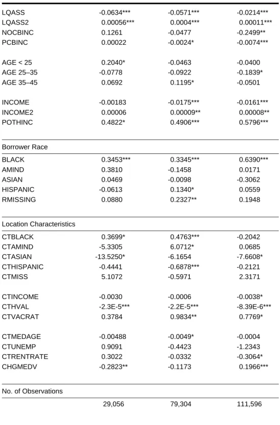
Table 3
Logit Estimations of the Cumulative Probability of Loan Default
1987 1988 1989
Loans Loans Loans
INTERCEPT -5.1785*** -4.8171*** -6.74*** Loan Characteristics LTV 4.1089*** 3.8381*** 6.1806*** HEI 20–38 0.2461** 0.1334* 0.1990*** HEI 38–50 0.5846* -0.0482 0.2176 HEI > 50 -0.3095 0.1501 1.7305** DTI 20–41 -0.0989 -0.0725 0.2008 DTI 41–53 -0.2118* -0.1649* 0.2192 DTI 53–65 -0.1644 0.1202 0.3684* DTI > 65 0.1671 0.1202 0.2383 REFIN 0.4474** 0.2932* 0.4078** CONDO 0.8118*** 0.3334** 0.4086** BUYDOWN 0.1482 0.0085 INVEST 0.0114 -0.0368 -0.4373
HVAL -8.7E-6 6.3E-6 -2.2E-5***
HVAL2 1.3E-12 -3.4E-11 1.3E-12***
DIRECT -0.2547 -0.4353*** -0.6767*** SHRTMOR -0.7898*** -0.4298*** -0.2726* URBAN 0.1576* 0.0749 0.0258 RURAL 0.0823 -0.0717 0.1001 HERF______ -0.0004** -0.0004*** -0.0004*** Borrower Characteristics COMP -0.0878 -0.0879 -0.0585 FIRSTBUY 0.0787 0.1930*** 0.0985* NEW -0.0338 -0.1231* -0.2177** CBUNMARD -0.1945 -0.0956 -0.0219 SINGLEM -0.0405 0.1326* 0.0753 SINGLEF -0.3051* -0.3015*** -0.3636*** SEPNUM 0.1847*** 0.1334*** 0.1767*** SELFEMP -0.5437 -0.2557 0.0915
Table 3 (continued)
LQASS -0.0634*** -0.0571*** -0.0214*** LQASS2 0.00056*** 0.0004*** 0.00011*** NOCBINC 0.1261 -0.0477 -0.2499** PCBINC 0.00022 -0.0024* -0.0074*** AGE < 25 0.2040* -0.0463 -0.0400 AGE 25–35 -0.0778 -0.0922 -0.1839* AGE 35–45 0.0692 0.1195* -0.0501 INCOME -0.00183 -0.0175*** -0.0161*** INCOME2 0.00006 0.00009** 0.00008** POTHINC 0.4822* 0.4906*** 0.5796*** Borrower Race BLACK 0.3453*** 0.3345*** 0.6390*** AMIND 0.3810 -0.1458 0.0171 ASIAN 0.0469 -0.0098 -0.3062 HISPANIC -0.0613 0.1340* 0.0559 RMISSING 0.0880 0.2327** 0.1948 Location Characteristics CTBLACK 0.3699* 0.4763*** -0.2042 CTAMIND -5.3305 6.0712* 0.0685 CTASIAN -13.5250* -6.1654 -7.6608* CTHISPANIC -0.4441 -0.6878*** -0.2121 CTMISS 5.1072 -0.5971 2.3171 CTINCOME -0.0030 -0.0006 -0.0038*CTHVAL -2.3E-5*** -2.2E-5*** -8.39E-6***
CTVACRAT 0.3784 0.9834** 0.7769* CTMEDAGE -0.00488 -0.0049* -0.0004 CTUNEMP 0.9091 -0.4423 -1.2343 CTRENTRATE 0.3022 -0.0332 -0.3064* CHGMEDV -0.2823** -0.1173 0.1966*** No. of Observations 29,056 79,304 111,596
Note: The symbols *, **, and *** denote statistical significance at the 90, 99, and 99.9 per-cent levels, respectively.
Simple bivariate correlations suggest that default probabilities differ significantly by loan, borrower, and location characteristics. For example, higher default rates appear to be associated with higher loan-to-value ratios, lower incomes and home values, and smaller loan amounts. Among racial and ethnic groups, the highest rates of loan default are associated with black borrowers, while Asian borrowers exhibit the lowest default rates. Default rates are also higher among borrowers residing in predominantly minority neighborhoods.10
Table 3 presents results of logit estimations of the relationship between the probability of default and a selected subset of independent variables.11 Results are provided separately for loans originated in 1987, 1988, and 1989.
The primary focus of this study is the effect of race and neighborhood characteristics on default, after controlling for other important determinants of risk. These results are dis-cussed here; other coefficient estimates are disdis-cussed in Berkovec et al. (1994, 1995). The residual effect of borrower race on default is estimated by including a series of dummy variables indicating that the borrower is black (BLACK), American Indian or Alaskan Native (AMIND), Asian (ASIAN), or Hispanic (HISPANIC), with whites repre-senting the omitted category. Because information on race was not coded for a number of loans, a dummy variable indicating that the borrower’s race or ethnic status is unknown (RMISSING) was also included.
The main result of the study is that, after controlling for the influence of other variables in the analysis, it was found that black borrowers exhibit a significantly higher likelihood of default than do white borrowers. For example, in the 1987 cohort, black borrowers are predicted to have cumulative default rates that are about 2 percentage points higher than those of white borrowers, all else being equal. This differential is smaller than the ob-served differential in default rates for the 1987 sample, in which the default rate for blacks is 9.0 percent, compared with a default rate for whites of 4.3 percent. Thus approximately one-half of the differential in observed default rates between whites and blacks can be explained by differences in other characteristics. Other years show similar results, al-though cumulative default rates for all racial groups are lower.12 Except for blacks, no other racial or ethnic group is found to be consistently different from whites in the likeli-hood of default, once other factors are taken into account.
As for the coefficients of the census tract variables, only a few consistent patterns are found. Focusing on neighborhood racial composition, we find some evidence of a positive relationship between the proportion of the neighborhood population that is black and the likelihood of default in the 1987 and 1988 cohorts, but the coefficient of CTBLACK is negative and statistically insignificant in the 1989 cohort.13 A somewhat more consistent pattern emerges with respect to the Asian and Hispanic populations of a neighborhood, since the coefficients of CTASIAN and CTHISPANIC are negative in all three cohorts and statistically significant—at a very modest level—for two of them.
Despite attempts to exploit the FHA data to the extent possible to control for the major determinants of loan performance that may be correlated with race or ethnic status, the possibility that such a variable has been omitted remains a concern. The most obvious candidate for such a variable is the borrower’s credit history, found by MBMT to be important in explaining the likelihood of a loan denial in the application decision process. In terms of the specific results obtained, the concern is that if black borrowers on average have worse credit histories than white borrowers, the greater likelihood of default ob-served for blacks may be attributable to differences in credit histories and may obscure any differential in default rates due to discrimination.
Although we cannot adequately account for credit history in the FHA data, we do attempt to measure the potential bias introduced by its omission from the model, as described in Berkovec et al. (1994). Our findings suggest that the coefficient of BLACK is system-atically biased upward—by as much as 40 percent—by the omission of credit history information. However, this is not enough to reverse the sign of the coefficient or influence its statistical significance.
Further checks on the robustness of the main results are described in Berkovec et al. (1994, 1995). These tests included separating the data into subsamples based on levels of risk or values of exogenous variables, with default models estimated separately for each subsample. The results indicate that the finding of higher default rates for black borrowers is not sensitive to a specific selection of data. Black borrowers exhibit significantly higher default rates in virtually all subsamples.
Data on the dollar value of losses are also examined (Berkovec et al., 1995). These results indicate that loss rates after default also tend to be higher for black borrowers. Differences in loss rates from default do not counteract the racial differences in default rates. Black borrowers appear to have higher overall default costs relative to other borrowers, condi-tioned on available loan characteristics.
Summary
Recent years have witnessed widespread allegations of racial discrimination in mortgage lending. A model of discrimination in credit markets suggests that discrimination carried out by setting higher qualification standards for minority applicants or applicants from minority neighborhoods may be revealed in differential performance of loans extended to these groups. This predicted effect of discrimination is the basis of the empirical tests used in this analysis.
The empirical results do not support a finding of widespread racial bias in mortgage lending. The main empirical finding is that, after controlling for a wide variety of loan, borrower, and property-related characteristics, default rates for black borrowers are higher than those for white borrowers. This finding is the opposite of the prediction of the model for lender bias against black borrowers.
Although the empirical finding of higher default rates for blacks in the FHA data appears to be quite robust, conclusions about discrimination are subject to several important caveats. First, omitted variables may bias the results away from finding the expected performance effects from discrimination.14 While we have sought to exploit the data as fully as possible in order to account for all relevant determinants of default likelihoods and losses, it is likely that some variables were omitted. We have attempted to estimate the magnitude of bias caused by the lack of credit history information in our data. Results do not appear to be altered substantively by the omission of credit history. However, this conclusion is tentative, and it is still possible that omitted variables, correlated with race or ethnicity, could affect the results.
Another caveat is that the basic theoretical prediction that discrimination results in better observed relative loan performance depends on the assumption that lending bias takes the form of different standards of creditworthiness for different groups. Other forms of dis-crimination that do not alter the distribution of accepted loans would not be revealed in a performance study such as this.
Finally, it should be noted that the model assumes that underlying “true” default prob-abilities, conditioned on creditworthiness factors observed by the lender, do not differ by race. Violation of this assumption, so that borrower race remains predictive of default even after controlling for creditworthiness, creates the potential for so-called “statistical” discrimination by lenders. This type of correlation between race and the “true” default rates could explain the empirical findings. Thus the estimation findings are not necessarily inconsistent with the existence of “statistical” discrimination.
Authors
James Berkovec is a senior economist at Freddie Mac; Glenn Canner and Timothy Hannan are senior economists in the Division of Research and Statistics, Board of Gov-ernors of the Federal Reserve System; Stuart Gabriel is a Professor of Finance and Business Economics in the Graduate School of Business Administration of the Univer-sity of Southern California.
Notes
1. The views expressed are those of the authors and do not necessarily reflect the views of the Federal Home Loan Mortgage Corporation, the Board of Governors of the Fed-eral Reserve System, or members of the Board’s staff. The authors are grateful to the Office of Policy Development and Research of the U.S. Department of Housing and Urban Development (HUD) for providing the FHA mortgage data utilized in this research. Special thanks go to William Shaw of the Office of Housing at HUD for his assistance.
2. As documented in recent analyses (see, for example, MBMT and Canner, Gabriel, and Woolley, 1991), minority loan applicants and neighborhoods are often character-ized by higher levels of default risk, relative to the applicant population as a whole. However, to the extent that loan underwriting requirements fully account for bor-rower and location default risk, and hence coincide with actual loan performance, applicant and neighborhood racial composition should play no residual role in the credit extension decision.
The settlement reached by the U.S. Department of Justice and Shawmut Mortgage Corporation (December 1993), for instance, noted that Shawmut had discriminated against minorities by holding them to a higher standard than those applied to white applicants. Shawmut was also accused of not giving minorities the same assistance provided to white applicants in overcoming borrowing obstacles. (For further discus-sion, see The Wall Street Journal, December 14, 1993.)
3. Evidence from MBMT appears to support the assumption about bias. The study indi-cates that, to the extent that differences in decisions about applications are observed, they appear in decisions concerning marginally qualified minority and nonminority applicants. MBMT notes that virtually all well-qualified applicants in their study— minority and nonminority alike—were approved for credit.
4. Commentaries in the media focus on ex post average default rates. (See, for example, “The Hidden Clue,” Peter Brimelow and Leslie Spencer, Forbes, January 4, 1991.) In doing so, those studies implicitly assume that the risk distributions of minority and majority borrowers are identical. However, evidence from MBMT and Canner, Gabriel, and Woolley (1991) indicates systematic variation in risk distribution among minority and majority borrowers.
5. To see this result, simply differentiate R with respect to B and B' as shown in Berkovec, Canner, Gabriel, and Hannan (1994).
6. It is also important to note that in this model, even though lenders know the true relationship between characteristics X and the probability of default and use the information in their underwriting, observed default rates will still vary with X. This does not necessarily mean that lenders could improve their performance by altering their underwriting rules.
7. This assumes that the distribution of ε does not depend on the borrower’s race. 8. The specific sections of the FHA mortgage insurance program examined in this study
are Sections 203, 234, 244, 248, 296, 303, 348, 503, 534, 548, and 596.
9. An earlier paper assessed the effects of a large number of additional neighborhood change variables on default probabilities and generally found little relationship be-tween these variables and the likelihood of default (Berkovec et al., 1994).
10. A detailed discussion of cumulative default rates by borrowers with these and other characteristics may be found in Berkovec et al. (1993).
11. The models contain about 100 independent variables. Space considerations preclude presentation of all estimates.
12. This is primarily due to the shorter loan lifetime from origination to the first quarter of 1993.
13. As a further test of the interaction between an individual’s race and neighborhood ra-cial composition, the sample was split into quartiles based on the percentage of minorities in the neighborhood, with default models estimated on each quartile sepa-rately. These results indicate that black borrowers have higher default rates in each type of neighborhood, since the magnitude of the coefficient of BLACK does not vary substantially among the quartiles and is significantly different from 0 in 10 of the 12 (4 runs each year in 1987–1989) logit analyses.
14. Since minorities tend to have riskier observed characteristics, it is likely that omitted unobserved characteristics for minorities also are riskier on average. The probable ef-fect of omitted variables in a default equation thus is to show higher defaults for minorities, a bias toward finding no evidence of discrimination. In accept/reject stud-ies, such as the one by MBMT, the probable bias of omitted variables goes the other way, toward finding discrimination.
References
Barth, James R., Joseph J. Cordes, and Anthony M.J. Yezer. October 1979. “Financial In-stitution Revolutions, Redlining and Mortgage Markets,” in The Regulation of Financial Institutions, Conference Series No. 21, Federal Reserve Bank of Boston.
Becker, Gary S. 1971. The Economics of Discrimination. (2d Edition) Chicago: Univer-sity of Chicago Press.
Berkovec, James A., Glenn B. Canner, Stuart A. Gabriel, and Timothy H. Hannan. May 1993. “Race and Residential Mortgage Defaults: Evidence from the FHA-Insured Single-Family Loan Program.” Conference paper prepared for the U.S. Department of Housing and Urban Development Conference on Discrimination and Mortgage Lending. Washing-ton, D.C.
______. November 1994. “Race, Redlining, and Residential Mortgage Loan Perfor-mance.” Journal of Real Estate Finance and Economics.
______. March 1995. “Discrimination, Default, and Loss in FHA Mortgage Lending.” Working paper.
Board of Governors of the Federal Reserve System. June 1991. “Feasibility Study on the Application of the Testing Methodology to the Detection of Discrimination in Mortgage Lending.” Staff analysis.
Canner, Glenn B., Stuart A. Gabriel, and J. Michael Woolley. 1991. “Race, Default Risk, and Mortgage Lending: A Study of the FHA and Conventional Loan Markets,” Southern
Economic Journal 58.
Canner, Glenn B., Wayne Passmore, and Dolores S. Smith. February 1994. “Residential Lending to Low-Income and Minority Families: Evidence from the 1992 HMDA Data,”
Federal Reserve Bulletin 80.
Clauretie, Terrence M. and Thomas Herzog. 1989. “The Effect of State Foreclosure Laws on Loan Losses,” Journal of Money, Credit, and Banking 22.
Ferguson, Michael F. and Stephen R. Peters. March 1995. “What Constitutes Evidence of Discrimination in Lending?” Journal of Finance, 50:739.
Lang, William W. and Leonard J. Nakamura. 1993. “A Model of Redlining,” Journal of
Urban Economics 33.
Munnell, Alicia H., Lynn E. Browne, James McEneaney, and Geoffrey M.B. Tootell. Oc-tober 1992. “Mortgage Lending in Boston: Interpreting HMDA Data.” Working Paper No. 92–7, Federal Reserve Bank of Boston.
Peterson, Richard L. Autumn 1981. “An Investigation of Sex Discrimination in Commer-cial Banks’ Direct Consumer Lending,” The Bell Journal of Economics 12.
Tootell, Geoffrey M.B. September/October 1993. “Defaults, Denials, and Discrimination in Mortgage Lending,” New England Economic Review.
Van Order, Robert, Ann-Margaret Westin, and Peter Zorn. January 1993. “Effects of the Racial Composition of Neighborhoods on Default and Implications for Racial Discrimina-tion in Mortgage Markets.” Paper presented at the Allied Social Sciences AssociaDiscrimina-tion meetings in Anaheim, California.
Yezer, A., R. Phillips, and R. Trost. October 1993. “Bias in Estimates of Discrimination and Defaults in Mortgage Lending: The Effects of Screening and Self Selection.” Unpub-lished paper. Department of Economics, George Washington University.