Data Analytics to Dissect Healthcare Delivery Patterns

Data Analytics to Dissect Healthcare Delivery Patterns

Luke Gallione

1250 14th St. Denver, Colorado 80202

[email protected]

Jack Schryver

Laboratory 1 Bethel Valley Rd Oak Ridge, TN 37831

[email protected]

Arjun Shankar

Laboratory 1 Bethel Valley Rd Oak Ridge, TN 37831

[email protected]

ABSTRACT

We systematically dissect and explain variation in Medicare costs by exploring the correlation structure in a recently re-leased set of Medicare data. A portion of regional variation in Medicare cost occurs due to geographic differences in pay-ment rates due to standard-of-living adjustpay-ments for individ-ual services. However, we are concerned with explaining the variance that remains after standardized cost adjustment. By relating the demographic, service utilization, and pre-vention quality indicator data to the standardized per capita Medicare costs (SPCC), we highlight key service usage pat-terns which explain the variance in cost. By taking this information into account, it should be possible to develop policy-driving recommendations that encourage more cost-efficient, high-quality medical care. We present a method to identify minimal multiple linear regression models which account for the most variance in Medicare cost. We then focus our attention on a model trained on data from 2007 which explains 95% of this variance with only five predic-tor variables. Finally, we discuss the results of this method across multiple years of data where we observe a shift of the predictors of SPCC from quantity of services to quality of services. Our contribution is a principled approach to de-construct a vital real-world data set that can better inform policy decisions about regional differences in Medicare costs and benefits.

1.

INTRODUCTION

The Center for Medicare and Medicaid Services (CMS) has released data which contains aggregated demographic, Medi-care spending, MediMedi-care utilization, and prevention quality indicator data consisting of over three hundred and fifty vari-ables for its three hundred and dix different Hospital Refer-ral Regions (HRRs) for four years starting in 2007 [8]. Our research explores the correlation structure underlying this data in an attempt to explain variation in Medicare costs, rather than the variables which overtly contribute the most to cost. The focus on variance allows us to highlight in-consistencies in spending and quality of healthcare delivery.

By understanding these inconsistencies and their sources, we hope to inform policy decisions which make Medicare more efficient. To our knowledge, no other prior work has taken a comprehensive and systematic look at the several hundred variable dataset to reduce it to a few relevant indicators.

The next section of the paper (Section 2) presents relevant background information including the definition of an HRR and the various measures of cost under consideration. We also use a simple heatmap of the correlation matrix to dis-cuss the ways in which indicators relate (and may vary) with each other. Section 3 describes the three step variable selec-tion process for a multiple linear regression model. Secselec-tion 4 discusses three standard linear regression diagnostics on this model. Section 5 is an analysis of the predictive performance of the model in time. Section 6 provides general conclusions and thoughts for future work.

2.

BACKGROUND

Thomas Bodenheimer’s excellent overview of the rising cost of healthcare in the United States essentially concludes that an aging population has only a small influence on cost growth. Instead, he finds that the spread of innovative technologies and a health system in which providers dominate the market explain the rise in expenditures. These factors are not unre-lated as he suggests: “when payers cured prices and quanti-ties of medical services in the early 1990s, hospitals consol-idated into systems that could command higher prices and fewer restrictions on quantities of services. Because most facilities for new technologies were located at hospitals, hos-pital market power enabled these technologies to prolifer-ate [1, 2, 3, 4].” These technologies promise improved quality of care if used appropriately. Therefore we should be hesi-tant to restrict their usage outright. Fisher and Wennberg et al. conclude that the average baseline health status of Medicare beneficiaries “was similar across regions of differ-ing spenddiffer-ing levels, but patients in higher spenddiffer-ing regions received approximately 60% more care[6, 7].” The increased utilization was explained primarily by three factors. First, more frequent physician visits, especially in the inpatient setting. Second, more frequent tests and minor (but not major) procedures. Third, increased use of specialists and hospitals. Interestingly, they also found no significant cor-relation between spending and access to care and between spending and quality of care. Thorpe and Howard conclude that virtually all of the growth in Medicare beneficiaries’ health care spending is associated with patients who are un-der medical management for five or more conditions [9]. Our

Figure 1: The 306 Hospital Referral Regions. Note that some locations are assigned to the Unknown HRR. This accounts for the holes in the map.

work responds to these above analyses using our encompass-ing approach that starts with all of the indicator data.

Hospital Referral Region Data

The HRR is a region with locality of medical referrals. HRRs have been defined by determining where patients were re-ferred for major cardiovascular surgery and neurosurgery consultations and procedures. The regions are generally larger than a county, but smaller than a state, and are shown in Figure 1. We analyze a dataset of aggregate data contain-ing the average values at the HRR level. This data set is cre-ated from a larger data set containing data at the individual level. This aggregate data does not contain any Personally Identifiable Information (PII) and has been made available to the public by CMS.

The data types are demographic, Medicare spending, Medi-care utilization, and prevention quality indicator data.

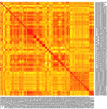
As an initial exploration into and description of this data set, consider the heatmap in Figure 2, which shows the relative level of correlation between 98 variables in 2007. The data are left in the order given by CMS: demographic, Medicare spending, Medicare service utilization, and pre-vention quality indicator data. The color red corresponds to complete positive correlation as can be seen by inspect-ing the main diagonal, while a color of white corresponds to complete negative correlation as can be seen by inspecting the variables “Percent.Female” and “Percent.Male”. Certain variables have a strong positive correlation with their neigh-bor. This is no coincidence. Many variables encode similar information. For example, the variables “Percent of Benefi-ciaries using Post Acute Care Home Health services,”“Post Acute Care Home Health Covered Stays,” and “Post Acute Care Home Health Covered Days” can be seen to correlate strongly with each other by observing a three by three red square on the diagonal of Figure 2. The other two by two and three by three red squares on the diagonal indicate other variables which contain similar information to each other.

The Medicare spending in a given HRR is specified by the value of the “Actual Cost” variable, but the CMS data set contains other measures of spending, including “Standard-ized Cost,”“Standard“Standard-ized Risk Adjusted Cost” and per capita versions of all three. The per capita values are the most

illu-Count.of .Beneficiar ies A v er age .Age P ercent.F emale P ercent.Male P ercent.Non.Hispanic.WhiteP ercent.Afr ican.Amer ican P ercent.Hispanic P ercent.Asian.Amer ican.P acific.Islander P ercent.Amer ican.Indian.Alaskan.Nativ e P ercent.Other ..Unkno wn P ercent.Eligib le .f or .Medicaid A v er age .HCC.Score P ercent.of .Medicare .beneficiar ies .who .ha v e .had.a.hear t.attack P ercent.of .Medicare .beneficiar ies .with.atr ial.fibr illation P ercent.of .Medicare .beneficiar ies .with.chronic.kidne y.disease P ercent.of .Medicare .beneficiar ies .with.chronic.obstr uctiv e .pulmonar y.disease P ercent.of .Medicare .beneficiar ies .with.depression P ercent.of .Medicare .beneficiar ies .with.diabetes P ercent.of .Medicare .beneficiar ies .with.hear t.f ailure P ercent.Medicare .beneficiar ies .with.ischemic.hear t.disease P ercent.of .Medicare .beneficiar ies .with.breast.cancer P ercent.of .Medicare .beneficiar ies .with.colorectal.cancer P ercent.of .Medicare .beneficiar ies .with.lung.cancer P ercent.of .Medicare .beneficiar ies .with.prostate .cancer P ercent.of .Medicare .beneficiar ies .with.asthma P ercent.of .Medicare .beneficiar ies .with.h yper tension Standardiz ed.P er .Capita.Costs IP.Users ..with.a.co v ered.sta y. X..of .Beneficiar ies .Using.IP IP.Co v ered.Sta ys .P er .1000.Beneficiar ies IP.Co v ered.Da ys .P er .1000.Beneficiar ies X..of .Beneficiar ies .Using.IP..IPPS IP..IPPS.Co v ered.Sta ys .P er .1000.Beneficiar ies IP..IPPS.Co v ered.Da ys .P er .1000.Beneficiar ies X..of .Beneficiar ies .Using.P A C X..of .Beneficiar ies .Using.P A C..IRF P A C..IRF .Co v ered.Sta ys .P er .1000.Beneficiar ies P A C..IRF .Co v ered.Da ys .P er .1000.Beneficiar ies X..of .Beneficiar ies .Using.P A C..SNF P A C..SNF .Co v ered.Sta ys .P er .1000.Beneficiar ies P A C..SNF .Co v ered.Da ys .P er .1000.Beneficiar ies X..of .Beneficiar ies .Using.P A C..HH P A C..HH.Episodes .P er .1000.Beneficiar ies P A C..HH.Visits .P er .1000.Beneficiar ies X..of .Beneficiar ies .Using.Hospice Hospice .Co v ered.Sta ys .P er .1000.Beneficiar ies Hospice .Co v ered.Da ys .P er .1000.Beneficiar ies X..of .Beneficiar ies .Using.OP OP.Visits .P er .1000.Beneficiar ies X..of .Beneficiar ies .Using.Outpatient.Dialysis .F acility Outpatient.Dialysis .F acility.Ev ents .P er .1000.Beneficiar ies X..of .Beneficiar ies .Using.FQHC.RHC FQHC.RHC.Ev ents .P er .1000.Beneficiar ies X..of .Beneficiar ies .Using.ASC ASC.Ev ents .P er .1000.Beneficiar ies X..of .Beneficiar ies .Using.EM EM.Ev ents .P er .1000.Beneficiar ies X..of .Beneficiar ies .Using.PR OC PR OC.Ev ents .P er .1000.Beneficiar ies X..of .Beneficiar ies .Using.IMG IMG.Ev ents .P er .1000.Beneficiar ies X..of .Beneficiar ies .Using.DME DME.Ev ents .P er .1000.Beneficiar ies X..of .Beneficiar ies .Using.LABTST LABTST .Ev ents .P er .1000.Beneficiar ies X..of .Beneficiar ies .Using.O THTST O THTST .Ev ents .P er .1000.Beneficiar ies X..of .Beneficiar ies .Using.PT .B.DR UG X..of .Beneficiar ies .Using.O THER Number .of .Acute .Hospital.Readmissions Hospital.Readmission.Rate Emergency.Depar tment.Visits Emergency.Depar tment.Visits .per .1.000.Beneficiar ies Hear t.attack.patients .giv en.aspir in.at.hospital.arr iv al Hear t.attack.patients .with.aspir in.prescr ibed.at.hospital.discharge Hear t.attack.patients .prescr ibed.angiotensin.con v er ting.enzyme .inhibitor .or .angiotensin.receptor .b lock er .at.hospital.discharge Hear t.attack.patients .with.smoking.cessation.counseling.dur ing.hospital.sta y Hear t.attack.patients .with.beta.b lock er .prescr ibed.at.hospital.discharge Hear t.f ailure .patients .with.discharge .instr uctions Hear t.f ailure .patients .with.e v aluation.of .left.v entr icular .systolic.function Hear t.f ailure .patients .prescr ibed.angiotensin.con v er ting.enzyme .inhibitor .or .angiotensin.receptor .b lock er .at.hospital.discharge Hear t.f ailure .patients .with.smoking.cessation.counseling Pneumonia.patients .with.pneumococcal.v accination Pneumonia.patients .with.appropr iate .initial.antibiotic.selection.f or .comm unity.acquired.pneumonia.in.imm unocompetent.patients Pneumonia.patients .with.b lood.cultures .in.emergency.depar tment.bef ore .antibiotic.administered Pneumonia.patients .with.influenza.v accination Pneumonia.patients .with.smoking.cessation.counseling Pneumonia.patients .with.initial.antibiotic.receiv ed.within.6.hours .of .hospital.arr iv al Surger y.patients .with.proph ylactic.antibiotic.receiv ed.within.one .hour .pr ior .to .surger y.incision Surger y.patients .with.appropr iate .proph ylactic.antibiotic.selection Surger y.patients .with.proph ylactic.antibiotics .discontin ued.within.24.hours .after .surger y.end.time Surger y.patients .with.recommended.v enous .thromboembolism.proph ylaxis .ordered Surger y.patients .who .receiv ed.appropr iate .v enous .thromboembolism.proph ylaxis .betw een.24.hours .pr ior .to .surger y.and.24.hours .after .surger y PQI11.Bacter ial.Pneumonia.Admission.Rate ..age .65.74. PQI08.CHF .Admission.Rate ..age .75.. PQI10.Deh ydr ation.Admission.Rate ..age .75.. PQI11.Bacter ial.Pneumonia.Admission.Rate ..age .75.. PQI12.UTI.Admission.Rate ..age .75.. PQI12.UTI.Admission.Rate..age.75.. PQI11.Bacterial.Pneumonia.Admission.Rate..age.75.. PQI10.Dehydration.Admission.Rate..age.75.. PQI08.CHF.Admission.Rate..age.75.. PQI11.Bacterial.Pneumonia.Admission.Rate..age.65.74. Surgery.patients.who.received.appropriate.venous.thromboembolism.prophylaxis.between.24.hours.prior.to.surgery.and.24.hours.after.surgery Surgery.patients.with.recommended.venous.thromboembolism.prophylaxis.ordered Surgery.patients.with.prophylactic.antibiotics.discontinued.within.24.hours.after.surgery.end.time Surgery.patients.with.appropriate.prophylactic.antibiotic.selection Surgery.patients.with.prophylactic.antibiotic.received.within.one.hour.prior.to.surgery.incision Pneumonia.patients.with.initial.antibiotic.received.within.6.hours.of.hospital.arrival Pneumonia.patients.with.smoking.cessation.counseling Pneumonia.patients.with.influenza.vaccination Pneumonia.patients.with.blood.cultures.in.emergency.department.before.antibiotic.administered Pneumonia.patients.with.appropriate.initial.antibiotic.selection.for.community.acquired.pneumonia.in.immunocompetent.patients Pneumonia.patients.with.pneumococcal.vaccination Heart.failure.patients.with.smoking.cessation.counseling Heart.failure.patients.prescribed.angiotensin.converting.enzyme.inhibitor.or.angiotensin.receptor.blocker.at.hospital.discharge Heart.failure.patients.with.evaluation.of.left.ventricular.systolic.function Heart.failure.patients.with.discharge.instructions Heart.attack.patients.with.beta.blocker.prescribed.at.hospital.discharge Heart.attack.patients.with.smoking.cessation.counseling.during.hospital.stay Heart.attack.patients.prescribed.angiotensin.converting.enzyme.inhibitor.or.angiotensin.receptor.blocker.at.hospital.discharge Heart.attack.patients.with.aspirin.prescribed.at.hospital.discharge Heart.attack.patients.given.aspirin.at.hospital.arrival Emergency.Department.Visits.per.1.000.Beneficiaries Emergency.Department.Visits Hospital.Readmission.Rate Number.of.Acute.Hospital.Readmissions X..of.Beneficiaries.Using.OTHER X..of.Beneficiaries.Using.PT.B.DRUG OTHTST.Events.Per.1000.Beneficiaries X..of.Beneficiaries.Using.OTHTST LABTST.Events.Per.1000.Beneficiaries X..of.Beneficiaries.Using.LABTST DME.Events.Per.1000.Beneficiaries X..of.Beneficiaries.Using.DME IMG.Events.Per.1000.Beneficiaries X..of.Beneficiaries.Using.IMG PROC.Events.Per.1000.Beneficiaries X..of.Beneficiaries.Using.PROC EM.Events.Per.1000.Beneficiaries X..of.Beneficiaries.Using.EM ASC.Events.Per.1000.Beneficiaries X..of.Beneficiaries.Using.ASC FQHC.RHC.Events.Per.1000.Beneficiaries X..of.Beneficiaries.Using.FQHC.RHC Outpatient.Dialysis.Facility.Events.Per.1000.Beneficiaries X..of.Beneficiaries.Using.Outpatient.Dialysis.Facility OP.Visits.Per.1000.Beneficiaries X..of.Beneficiaries.Using.OP Hospice.Covered.Days.Per.1000.Beneficiaries Hospice.Covered.Stays.Per.1000.Beneficiaries X..of.Beneficiaries.Using.Hospice PAC..HH.Visits.Per.1000.Beneficiaries PAC..HH.Episodes.Per.1000.Beneficiaries X..of.Beneficiaries.Using.PAC..HH PAC..SNF.Covered.Days.Per.1000.Beneficiaries PAC..SNF.Covered.Stays.Per.1000.Beneficiaries X..of.Beneficiaries.Using.PAC..SNF PAC..IRF.Covered.Days.Per.1000.Beneficiaries PAC..IRF.Covered.Stays.Per.1000.Beneficiaries X..of.Beneficiaries.Using.PAC..IRF X..of.Beneficiaries.Using.PAC IP..IPPS.Covered.Days.Per.1000.Beneficiaries IP..IPPS.Covered.Stays.Per.1000.Beneficiaries X..of.Beneficiaries.Using.IP..IPPS IP.Covered.Days.Per.1000.Beneficiaries IP.Covered.Stays.Per.1000.Beneficiaries X..of.Beneficiaries.Using.IP IP.Users..with.a.covered.stay. Standardized.Per.Capita.Costs Percent.of.Medicare.beneficiaries.with.hypertension Percent.of.Medicare.beneficiaries.with.asthma Percent.of.Medicare.beneficiaries.with.prostate.cancer Percent.of.Medicare.beneficiaries.with.lung.cancer Percent.of.Medicare.beneficiaries.with.colorectal.cancer Percent.of.Medicare.beneficiaries.with.breast.cancer Percent.Medicare.beneficiaries.with.ischemic.heart.disease Percent.of.Medicare.beneficiaries.with.heart.failure Percent.of.Medicare.beneficiaries.with.diabetes Percent.of.Medicare.beneficiaries.with.depression Percent.of.Medicare.beneficiaries.with.chronic.obstructive.pulmonary.disease Percent.of.Medicare.beneficiaries.with.chronic.kidney.disease Percent.of.Medicare.beneficiaries.with.atrial.fibrillation Percent.of.Medicare.beneficiaries.who.have.had.a.heart.attack Average.HCC.Score Percent.Eligible.for.Medicaid Percent.Other..Unknown Percent.American.Indian.Alaskan.Native Percent.Asian.American.Pacific.Islander Percent.Hispanic Percent.African.American Percent.Non.Hispanic.White Percent.Male Percent.Female Average.Age Count.of.Beneficiaries

Figure 2: A heatmap showing the relative level of correlation between 98 variables in 2007. The data are left in the order given by CMS: demo-graphic, Medicare spending, Medicare service uti-lization, and prevention quality indicator data. Red, yellow, and white correspond to correlation coeffi-cient values of 1, 0 and -1, respectively.

minating since they do not depend on the number of Medi-care beneficiaries in a given HRR. The standardization is performed in order to remove geographic differences in pay-ment rates for individual services as a source of variation. This allows the utilization of services and their costs to be compared. For these reasons this investigation attempts to optimize a multiple linear regression on the “Standardized Per Capita Costs” (SPCC) variable.

3.

MULTIPLE LINEAR REGRESSION

VARI-ABLE SELECTION

The variable identification and parsimonious selection pro-cess involves three distinct phases: a pre-selection phase eliminates variables from the data set based on irrelevance, redundancy, and missing-data-driven simplifications, the sec-ond phase further winnows the list of variables by use of a recursive algorithm, and the third and final phase is an ex-haustive comparison of all linear models producible from the remaining variables. We focus our attention on the results of this method applied to the data from 2007, and investigate the applicability of the method and the insights it produces on the 2008-2010 data sets.

3.1

Pre-Selection

The initial data set consists of 359 variables for 306 different HRRs; however, many of these variables are redundant or irrelevant to our investigation. To begin, only cost variables which contained standardized costs were included since we are trying to predict SPCC solely from demographic, ser-vice utilization, and quality indicator variables. This left a remainder of 164 variables. We eliminated variables with count data, since we are concerned with per capita usage rather than totals. We also eliminated Average HCC Score Expressed as a Ratio to the National Average as it is a con-stant multiple of another variable, and is thus redundant in the context of linear regression. This brought the vari-able count down to 128. A final step eliminated all varivari-ables with missing values in any of the four years. This step is necessary, but may introduce bias. The final step succeeded in bringing the variable count down to 98. (Indeed these are the same 98 variables in Figure 2. The only Medicare spending variable in the heatmap is SPCC.)

3.2

Backwards Algorithm

After pre-selection a simple multivariate regression was per-formed using SPCC as the desired output and all 98 vari-ables as predictors. Then, the full model’s Akaike informa-tion criterion (AIC) was calculated. The AIC is a measure of the relative quality of a statistical model for a given set of data. Given a set of candidate models for the data, the preferred model is the one with the minimum AIC value. The AIC is defined by AIC = 2k−ln(L) wherek is the number of parameters in the model andLis the maximized value of the likelihood function for the model, which is pro-portional to the goodness of fit. Thus, the AIC deals with the trade-off between the goodness of fit of the model and the complexity of the model.

After the full model’s AIC was calculated, the predictor that contributes the least to the AIC was removed. A new model was fit to the remaining variables and the process was re-peated until removing a variable no longer lowers the AIC.

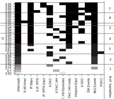
Figure 3: Variables for the top four models for mod-els with up to 7 predictors. The R2 _{value for each} model is shown on the y-axis, while a black rect-angle indicates that a particular x-axis variable is included in the model as a predictor. It is impres-sive that so few variables can account for nearly all of the variance in cost.

This “backwards” algorithm is in contrast to a “forwards” algorithm which would build the model up from an empty model. When this “backwards” algorithm was used on our 98 variables, the minimal AIC model was found when only 44 variables remained. While an exploration of these 44 vari-ables would be fruitful, the number of varivari-ables is unwieldy.

3.3

Exhaustive Comparison

The final step of variable selection compared the models whose predictors correspond to every subset of our remain-ing variables up to a maximum subset size of 7 predictors. The predictors for the top four models byR2_{value for each}

variable subset size are shown in Figure 3.

Note that the variables “IP.Stays” (In-Patient Covered Stays per 1000 Beneficiaries), “PAC..HH.Visits” (Post Accute Care Home Health Visits per 1000 Beneficiaries), and “IMG.Events” (Imaging Events per 1000 Beneficiaries) appear in the top 4 models for all models with at least 4 predictors. This is a strong indication that these variables consistently explain different aspects of the variance in SPCC. In Section 5 we shall focus on the variables that appear in the top models, rather than focusing on a single model. We believe that this approach offers deeper insight into our data’s corre-lation structure while also avoiding some of the pitfalls of over-fitting.

Despite this belief, and in order to keep our results tangi-ble, in Section 4 we have chosen to focus our attention on the optimum model with five predictors. The number five was chosen since the value of the coefficient of determination does not increase when the number of variables is increased from five to six; producing a distinct “elbow” on an elbow

Predictors Coeff. Stand. C. t value P(≥ |t|) Intercept 784.3 -1.364e-16 0 1 IP Stays 7.243 .2917 14.065 2e-16 % PAC 9867 .2669 10.524 2e-16 PACHH Visits .08773 .2886 14.263 2e-16 % ASC 3062 .1093 7.477 8.44e-13 IMG Events .6860 .3207 15.072 2e-16

Table 1: Standardized coefficients and t-test in-formation for five predictor variables for a multi-ple linear regression model trained on data from 2007. The variables are: “IP.Stays” (In-Patient Cov-ered Stays per 1000 Beneficiaries), “% PAC” (Per-centage of Beneficiaries using Post Acute Care per 1000 Beneficiaries), “PAC..HH.Visits” (Post Accute Care Home Health Visits per 1000 Beneficiaries), “% ASC” (Percentage of Beneficiaries using Ambu-latory Surgery Centers per 1000 Beneficiaries), and “IMG.Events” (Imaging Events per 1000

Beneficia-ries)

plot of number of variables vs. R2 value. The five predic-tors involved in the model are “In-Patient Covered Stays per 1000 Beneficiaries,” “Percent of Beneficiaries using Post Acute Care,”“Post Acute Care Home Health Visits per 1000 Beneficiaries,” “Percent of Beneficiaries using Ambulatory Surgical Centers,” and “Imaging Events per 1000 Beneficia-ries.” Note that even though demographic and prevention quality indicator variables were included in the initial data, our method primarily selects service utilization variables. The predictors are respectively abbreviated as “IP Stays,” “% PAC,”“PACHH Visits,”“% ASC,” and “IMG Events” for

the readability of Figures 3 and 4.

4.

MULTIPLE LINEAR REGRESSION

DI-AGNOSTICS

4.1

Standardized Coefficients

The actual values of the regression coefficients are not very informative. The standardized coefficients are the estimates resulting from an analysis carried out on independent vari-ables that have been standardized so that their variances are unity. Therefore, the standardized coefficients represent how many standard deviations SPCC will change for every standard deviation increase in the predictor variable. This allows the relative amount of variance in SPCC explained by each predictor to be compared, regardless of the units of the predictors. One must be careful to realize that an increase by one standard deviation has no reason to be “equivalent” to a similar change in another predictor, but conversely, that this method at least allows a baseline comparison to be made. A quick glance at Table 1, shows that four of the predictors, with standardized coefficients of about 0.3, explain roughly the same amount of variance. In contrast, when the value of the fifth predictor, “% ASC,” is increased by its standard de-viation, with all other variables held fixed at their average, the value of SPCC will only change by about 0.1 standard deviations. It is interesting to note that of the five included predictors in this model, “Percent of Beneficiaries using Am-bulatory Surgical Centers” was the least justifiable according to the variable selection process. In general though, these differences are negligible and it is sufficient to say that the

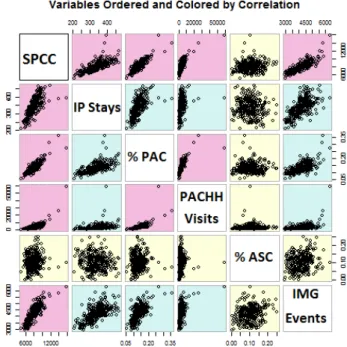
Figure 4: Scatterplot matrix of SPCC and the five predictor variables from 2007. The plotted variables in the pink, blue, and yellow panels have correspond-ing correlation coefficient values greater than .7, be-tween .3 and .7, and less than .3, respectively. The correlation matrix is symmetric.

five variables explain the same order of magnitude of vari-ance in SPCC.

4.2

T-Tests

The AIC does not provide a test of a model in the sense of testing a null hypothesis; i.e., AIC can tell nothing about the quality of the model in an absolute sense. If all the candidate models fit poorly, AIC will not give any warning of that. Therefore we consider the standard student’s T-test under the null hypothesis that the value of the coefficient is 0, that is, that the predictor and SPCC are not linearly related.

The second to last column of Table 1 contains the t-values for each predictor under this null hypothesis. The final column displays the probability that the measurement of all poten-tial t-values (which follow a t-distribution with 300 degrees of freedom and mean 0) is greater than the observed t-value given that the null hypothesis is true. This measure is com-monly referred to as a p-value. The estimated coefficients for four of the predictors are equally improbable under the null hypothesis. The probability value associated with “% ASC” is only slightly greater. These differences are negligible and since all five p-values are small it is sufficient to reject the null hypothesis that the value of the regression coefficient for each of the five predictors is 0. Thus the correlation between the five predictors and SPCC is statistically significant.

The scatterplot matrix in Figure 3 compares the values of SPCC and the five predictor variables from 2007. Four of the variables have a strong linear correlation with cost. The fifth variable, “% ASC” has almost no correlation with SPCC. Re-call that this model has anR2value (a measure of variance explained by the model) of .95. It is impressive that five variables can account for nearly all of the variance in cost.

5.

MODEL VALIDATION AND TEMPORAL

ANALYSIS

We now turn our attention to the results of this method across multiple years of data. First, the data was purged of all cost and total count information. As before, we also eliminated all variables with missing values in any of the four years. Then we applied the backwards algorithm to the remaining 98 variables. Between 40 and 50 variables remained, depending on year. Finally, the exhaustive com-parison step was applied. We once again decided to look at models with 7 or fewer predictors and only consider the four models within each predictor subset size with the highestR2

value.

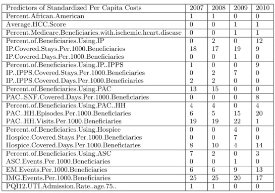
As mentioned above, it is somewhat misleading to focus on only the “top” model. Instead, it is wiser to analyze the top models as a group. Rather than displaying the graphic in Figure 3 for the remaining three years, we have summa-rized the information in Table 2. Note that the 2007 column matches the totals found in Figure 3.

A few significant trends emerges from this table. First, there is a shift from “Post Acute Care Home Health Visits” to “Post Acute Care Home Health Episodes.” Second, there is a shift from “In-Patient Covered Stays” to “percent of Benefi-ciaries using In Patient services.” Since there can be multiple visits within an episode, and since a beneficiary who uses IP services can have multiple stays, both of these trends may suggest an evolution of the predictors from quantity of ser-vices to quality of serser-vices. To a lesser extent this trend is present in the “Acute Inpatient Prospective Payment Sys-tem” (IPPS) variables as well. The prevalence of IP services as top predictors for SPCC supports the findings of Fisher and Wennberg et. all who claim that utilization in higher spending regions is partially “explained by more frequent physician visits, especially in the inpatient setting [6, 7].

However, we also notice an increase in the predictive power of Evaluation and Management Events, Skilled Nursing Fa-cility Covered Days, and Hospice Covered Days. The studies of Bodenheimer and of Fisher and Wennberg et. all claimed that hospital market power and increased utilization of hos-pitals and specialists were primary cost drivers [1, 2, 3, 4, 6, 7]. Our results do not support their findings since skilled nursing facilities and hospices are by definition not hospitals, but rather post-accute care facilities.

The number of Imaging Events is consistently a top predic-tor of SPCC for all four years of data. This corroborates the findings of Bodenheimer who claims that the spread of technology is a primary cost driver [1, 2, 3, 4]. This also cor-roborates the findings of Fisher and Wennberg et. all who claim that utilization in higher spending regions is partially explained by tests and technology events, and who further found that the “quality of care in higher spending regions

Average SPCC $8,216 $8,635 $9,044 $9,236 % growth of SPCC N.A. 1.051 1.047 1.021

Table 3: Average Standardized Per Capita Costs for 2007-2010. National SPCC as proportion of previ-ous year’s SPCC. While the result cannot be statis-tically significant with a sample size of only 3, note that 2010 has the least increase in SPCC.

was no better on most measures and was worse for sev-eral preventive care measures [6, 7].” We have observed that Prevention Quality Indicator data is not a top predictor of SPCC, which supports their claim.

Table 3 shows Average Standardized Per Capita Costs for 2007-2010 and National SPCC as percentage of previous year’s SPCC. While the result cannot be statistically sig-nificant with a sample size of only 3, note that growth rates appear to decline, and that 2010 has the least increase in SPCC.

6.

DISCUSSION AND CONCLUSION

Medicare provides legitimate services to millions of Ameri-cans, and any efforts to reduce cost should always be cou-pled with an effort to increase the quality of care. If one’s motivation is to blindly decrease overall Medicare spending without concern for the quality of care, then one is con-cerned with the variables which contribute the most to cost; the largest slices of pie on a pie chart. But if the motivation is to increase the efficiency of Medicare by removing what are deemed to be spending inconsistencies, then we are more concerned with the variation in cost than the values of cost. Recall that even though demographic and prevention qual-ity indicator variables were included in the initial data, our method selects service utilization variables as the primary explanation of variance in SPCC.

Our analysis is built on multiple linear regression modeling, which always comes with the caveat that correlation does not imply causation. Nevertheless, we believe that it is im-portant to understand the correlation structure of Medicare service utilization as it relates to standardized per capita costs (SPCC). For future work, we are investigating a struc-tural equation model for SPCC. Another caveat is that our linear modeling neglects non-linear relationships. We would also like to find a better way to deal with variables with miss-ing values. While not SPCC related, Cooper et. all found steep, curvilinear relationships between lower income and both increased hospital utilization and increasing percent-ages of individuals reporting disabilities [5]. Therefore we suspect that there may be important non-linear relation-ships to SPCC in our dataset.

Our results support previous findings that the spread of technology is a primary cost driver in the U.S. While in patient treatment is still an important cost driver, we have also observed a shift in predictors of SPCC towards evalua-tion and management events and post acute care facilities in the form of skilled nursing facilities and hospice treatment.

Perhaps the most interesting result is the shift of the pre-dictors from quantity of services to quality of services. This

Predictors of Standardized Per Capita Costs 2007 2008 2009 2010 Percent.African.American 1 1 0 0 Average.HCC.Score 0 0 1 1 Percent.Medicare.Beneficiaries.with.ischemic.heart.disease 0 0 1 1 Percent.of.Beneficiaries.Using.IP 0 2 0 12 IP.Covered.Stays.Per.1000.Beneficiaries 18 17 19 9 IP.Covered.Days.Per.1000.Beneficiaries 0 0 1 0 Percent.of.Beneficiaries.Using.IP..IPPS 1 0 0 9 IP..IPPS.Covered.Stays.Per.1000.Beneficiaries 0 2 7 0 IP..IPPS.Covered.Days.Per.1000.Beneficiaries 2 2 0 0 Percent.of.Beneficiaries.Using.PAC 13 15 0 0 PAC..SNF.Covered.Days.Per.1000.Beneficiaries 0 0 0 8 Percent.of.Beneficiaries.Using.PAC..HH 4 4 0 4 PAC..HH.Episodes.Per.1000.Beneficiaries 6 5 15 20 PAC..HH.Visits.Per.1000.Beneficiaries 19 19 22 1 Percent.of.Beneficiaries.Using.Hospice 0 0 4 0 Hospice.Covered.Stays.Per.1000.Beneficiaries 0 0 7 0 Hospice.Covered.Days.Per.1000.Beneficiaries 8 10 4 14 Percent.of.Beneficiaries.Using.ASC 7 2 0 3 ASC.Events.Per.1000.Beneficiaries 0 0 1 0 EM.Events.Per.1000.Beneficiaries 6 6 9 13 IMG.Events.Per.1000.Beneficiaries 25 25 20 17 PQI12.UTI.Admission.Rate..age.75.. 1 1 0 0

Table 2: Total number of models each variable is present in for the top four models for variable subset sizes 1 through 7 for four years of data. Observe that there are only three demographic variables and only one prevention quality indicator variable in this table, while the rest are service utilization variables. Note that the 2007 column matches the totals found in Figure 3. IP:In Patient. IPPS: Accute In Patient Prospective Payment System. PAC: Post Accute Care. SNF: Skilled Nursing Facility. HH: Home Health. ASC: Ambulatory Surgery Center. EM: Evaluation and Management. IMG: Imaging. UTI: Urinary Tract Infections.

coupled with the results in Table 3 suggest that the in-dustry’s attempt to switch from fee-for-service to pay-for-performance may be working. If this trend continues, then we expect to see a further decline in SPCC as a percentage of the previous year’s SPCC.

7.

REFERENCES

[1] T. Bodenheimer. High and rising health care costs. part 1: seeking an explanation.Annals of Internal Medicine, 142(10), 2005.

[2] T. Bodenheimer. High and rising health care costs. part 2: technologic innovation.Annals of Internal Medicine, 142(11):932–937, 2005.

[3] T. Bodenheimer. High and rising health care costs. part 3: the role of health care providers.Annals of Internal Medicine, 143(1):26–31, 2005.

[4] T. Bodenheimer and A. Fernandez. High and rising health care costs. part 4: can costs be controlled while preserving quality? Annals of Internal Medicine, 142(10):847–854, 2005.

[5] R. Cooper, M. Cooper, E. L. McGinley, X. Fan, and J. T. Rosenthal. Poverty, wealth, and health care utilization: A geographic assessment.Journal of Urban Health, 89(5):828–847, 2012.

[6] E. Fisher, D. E. Wennberg, T. A. Stukel, D. J.

Gottlieb, F. L. Lucas, and . L. Pinder. The implications of regional variations in medicare spending. part 1: The content, quality, and accessibility of care.Annals of Internal Medicine, 138(4):273–287, 2003.

[7] E. Fisher, D. E. Wennberg, T. A. Stukel, D. J.

Gottlieb, F. L. Lucas, and . L. Pinder. The implications of regional variations in medicare spending. part 2: Health outcomes and satisfaction with care.Annals of Internal Medicine, 138(4):288–298, 2003.

[8] C. for Medicare & Medicaid Services. Research, statistics, data & systems, June 2014.

[9] K. Thorpe and D. Howard. The rise in spending among medicare beneficiaries: the role of chronic disease prevalence and changes in treatment intensity.Health Affairs, 25(5):w378–w388, 2006.