Stats Notes.pdf

(1)

I

Mean and standard deviation

f

hiiii in. vs iv un in hhnii iLhtl lh.

ntnt ii iii.in inlies Iii iwn isiiiga gri1ih ,iIIuuI ‘t’igit’iiiV iistiihiitiuii ,\ti,sIs,iri,itiniigI5’ ,i _{luiIIsliuiitiI}

i’i_{0 em}_y istt hiit iiiii i lii Ithi’ tiornial distribution [he wean valueis in the inn kilo 0Ow Iistrihutii)n [1w meanof a

a viluius is ii.nlitniliiydiviuiniilthe sum 1,1the v,iliins iii. nuniliur ii viInts

Iiii i intili,thi2 Wifliii1110ViltiOS7, 0, I i1(i / is -Il md is

there ire our Values, liii’nle,in iv44 liiViiii’d by 3, whe 11 5

ii. slanilard devi.ttionis _{usuul to} issuSs mw tar h.- values -ire ‘.inewl ,iiiiuv. md Ii.lnvv lie neifl It is< iiiulatud liv

roteinig ilita mlii a griihic uiispiiv orvi entiticCalculitor md iressnugthestandard ileviati mtunition key. A high

taiimIirulmivmitiumnsI vvs hit thediii iii’wiiulv spiid, ‘uliuruis i luw‘tmiiimmiilivmitliimi ii, Ws hit tinujiti in

kistu i’d I u’,cl\’ ironiiii lii. niein

iii’‘t,iiid,iiuI(iivi,itiuiiii,iiiIii ti%(’ullii tilt, ilec iii’whi’)Iii’i j hi lilkr’iim u hu’twu’nn iwmi nu’,insi lik’ls to h sig;iliii ,itit

[‘Sm _{‘s,nnImlus n} liiiihiul Imuli

LEFT AND RIGHT HAND LENGTHS

lhmmtv tumiumgm lmuv’ niu,numu’mlthe In/h ni tliuir kit

Iiinmis, in mdmiii vImutliur thuv me ililturunt Indis ilnil inn,’

lilt miniright hunt length vu ed by is miii Ii is I i)mnm

liii ustilts ire shim iwn in tIn IrivIninc v iii’.trihnitmnii huh mw

hand Mean length Standard

deviation

hit )iBi,inimi It him

In’inuii

HAND AND FOOT LENGTHS

Flie‘nile tlmtv liunige ins, who neitinil ilnir hind

kinghis il-i ni,i’,nrmd h 10/Il ii their right nit. in mid

nIt ‘shiu’tlur 1 wi ihitlurunt rim tlirlinml length Iii’ iisoIts ire ‘.lniwn it the ieqneilivilistril iiition

ii

1 i

-deviation

right hind I 1111 4 miii Iii 1 mm

hohHii:OunmiItInIn_j

In

haiiil iiglit

I LLLLE

I ri) lit 100 Ii) 2Ii) 100 100 1)10

Iength,‘ inn

oil 70 Ill)) 110 200 210 _{13.-c iusc} _he_{st i0/}_iid_Ci(Vi_hums _{lit flhlit}_{h k ss lIt in thi}

I t,ini I Fm ngth/111 Cl _{ml Iterenci in mei}_n_length. I us vu ry ikel yIh,m 1 the ci terenc e n

mean length I metsveen rimht lii ndsaiimI rightbet issignificant.

let,m use tliest,iin ard deviationsare iii ush grea Icr than the ditterence in mean length, it is very unlikely thit the difference in mean length hetween left mci right hands is sugnitucant.

the normal distribution

A nsm’ttil rule istli,it (41/, ot lie v,ilni’s lie wlihin nite stnuml,nil

bevi,ijun mt thu mom in a mm nib listril nilion mud ittiimm’nniiulv‘i ii him v,ilnes Iii vvitlnn ism‘imimlmril levmitiuins m itthin niem ,ihuuvii

ii iii,iri

tt-1(4(1 (sn

Isv. ri I

.1-‘. iii’

ERROR BARS

(2)

Relationships

—

significance

and cause

tH t-TEST

I In he H OV 90(5 pa e, ins 0‘0100 fanI levtat u>0%we10 ((‘OH

lo .sses% whether I tOrI ices between ens were bkely to be go ic ant. 1) bgists >nen >eed to Inc Idemore >biectively

whether ditferenuns between means ne signOicant. ()ne of

be on151 frequent y used

methods

is ciiledthe ttest

the -lest can be used to find out whether there is a

significant difference between the means of two populations.

A htternoce s coosnlere( I statisticallysgn0icInt 1 he

>o iba hi ty >t tbeing due to rimlorn vartation s% ir tess,

Cs a statistic thatiscalculated(rum the twosets 01 measurements. [he larger the htference between thetwo

r mans, the arger t s, [be ar ger the staiiiIa rd 1ev at ions, the smallertis. It is not necessaryto earn how to calculatet,

becausea graphic display calculator or computer is nearly alwaysnoIC5(’d,

stages in using the Itest

Er ocr the values in.i grap ic displaycalculator or a

‘.preadsheet program, withvalues for the two populations

‘ntererl separately.

1. Use the calculator (unction keys or computer sottware to

calculatet,

1. Hod the number01degrees of treedom, [his will he the total number ot values in both populations, minus Iwo.

1. 1-md the critical value br feither using computer sottware or a table of values oft, ihe level ot significancetI

hosen should be005 (5%l and the appropriate row ‘,bould he selected according to the number of degrees of freedom,

5. Compare the calculated value oftwith the cntical value,

lithe critical value is exceeded, there is evidence of a

significant difference between the means, at the 5% level,

rable of critical values of I

Ii ‘vel of sgn (k-a nce(Pt

02 0.1 005 002 001 0.002

I 3078 6314 12 706 31 821 83657 318310

2 I $86 2320 4303 6 365 9.925 27327

3 1638 2.353 31112 4541 5841 10215

4 1533 2132 2776 3747 4604 7173

5 478 2015 2.571 3365 4032 5893

2 6 I440 I 043 2447 3143 3707 5208

cO 7 1415 I 1195 2385 2998 3,499 4.185

>1 I 397 1 1160 2.308 21396 3.355 4501

) 9 1 383 I833 2262 2 821 3250 3297

10 1372 1812 2228 2.764 3169 4.144

II 1363 1736 2201 2718 3,106 4025

12 1358 t 782 2.179 2681 3055 3930

l.> 13 1350 t 771 2.180 2.650 3.012 3.852

14 1345 1.781 2.145 2.624 2977 3.787

(5 I341 1 753 2)31 2.602 2.947 3.733

IS I 337 1,748 2.120 2.583 2.921 3686

17 1333 1.740 2.tIO 2.567 2.898 3.646

IS 1.330 1 734 2.101 2.552 2878 3.610

19 1.328 1729 2093 2.539 2.861 3.579 20 I325 t.725 2.086 2.528 2.845 3.552

30 1.310 I697 2.042 2.457 2.750 3.385

30 1 303 1.684 2.021 2.423 2.704 3.307

Examples of the use of the ttest

I Imse n’s a nples a re based on the lata r ha iid and lIt

b‘tigths lesc o bed (In the >revn10% Iage,

Festtng the Il(tterenue between mean lengths((1lOft and

light hands

Meanlength of left hands 108.6mm

Meanlengthof right hands = I88.4mm =0082

(ritical value for t= 2.002 IP 1)05)

[be calculated value of(is much smaller than the critical

value, sothe difference between themean lengthst>f left and r>ght hands is not significant.

2, festing the ddference between the mean lengths(Ifright hanrls ,ind right feet.

Mean length of right hatids= 1(18.4mm Me,n length of rIghtteet 262.3mm

Critical value fort= 2.005(P=0.05)

[be calculated value of tis much larger thao the crittcal

value, showing that the (lifterence between themeanlengths

(If ha oils a rid feet(Ssignificant.

In these two examples, the t-test confirms conclusions that are

reasonably obvious. In biological research, it is often much

less clear whether differences between means are significant

and the ttest is therefore very useful.

CORRELATION AND CAUSE

[he scattergraph heluw shows that there is a positive (‘orrelation between the lengths of the right hand.and right

lent of thirty teenage boys boys with larger hands tend to have larger teet as well.

290

2111)

- 270

260

250

241)

2.tt)

.t2t)

200

I0 170 180 I 90 200 21t) 220

Hand length / mm

Although there is a positive correlation between hand and foot length, we know that increases in the length of the hand do not cause increases in length of thetoot Instead, both are due to

the factors that control growth in teenage hoys. Ibis mistake is often made in analysis of data—a correlation between two

(3)

3tcittical hypothesis tests

ypothesis tests

A hypothesis rest

is

a statistical procedure for deciding whether

or

not to reject a “default belief”, known as a null hypothesis. The

decision is based on th

5 result

of a calculation, using the data that

you collected as the results of your experiment. Hypothesis tests

have the following key stages.

The hypotheses, H and H: H, stands for the null hypothesis,

and is the belief that there is nothing out of the ordinary (e.g.

the two means are equal, or there is no correlation). H, stands

for the alternative hypothesis, and is the belief that there is

something going on (e.g. the two means are different or there is

a positive correlation).

a

_{The significance level and critical region: the significance level}

is a somewhat arbitrary number, usually chosen to be 5 per cent.

It

is actually the probability of rejecting H

0 when H

0 is in fact

true, Obviously, we want this probability to be small

—

but make

it

too small and you are unlikely to reject H

0 when it is false! In

most cases, 5 per cent is fine. Most of the worked examples on

the following pages use this value. The critical region depends on

your significance level and the type of test. The critical region is

found either by using statistics tables or by a statisifcs program

on your computer. When you have done the calculation,

YOU

compare the calculated statistic with the critical region. If the

result

of your calculation lies in the critical region, H,, is rejected.

The data: it is good practice to include only a swmmary of the

data where you show the hypothesis test in your extended essay.

A suitable summary consists of as the number of observations

(n),

the mean

(x),

variance (S

2 ) and so on.

• The calculations: a formula is used to calculate a statistT.

Obviously

you must use the correct formula for the test that you

are using, and do the calculation without any mistakes. The

statistic is then compa red with the critical region.

The conclusions: in this last section you state whether there is

evidence to reject H

0 , and interpret the decision in the context of

your experiment.

One and twotailed tests

In all hypothesis tests you are likely to come across (except ANOVA),

you will have to decide whether a one-tailed or a two-tailed

test would be more appropriate. If, according to your alternative

hypothesis, one mean will be a largr than the other, or that the

correlation will be positive, you should do a one-tailed test. This type

of

test is only concerned with extreme results on one side. If you do

not know before you collect your

data

which mean will be larger than

the other or whether the correlation will be positive or negative, you

should do a two-tailed test. This test looks out for extreme values

on both sides. Note that in a one-tailed test, H, has a

sign, but in a

two-tailed test, I-I, has a <sign or a

>

sign.

1I

J

Most hypothesis

the calculation of a mean

variance or standard

In case you are not

fami

these, the formulae

are

below.

The mean

where E is the sum of.

In

Excel, this can be calculated

with the AVERAGE Function.

For example, AVERAGE (A2:A21)

calculates the mean of the values

in the cells A2 to A21.

The variance

—2

S

2 n—I

In Excel, use the VARP function.

For example, VARP(A2:A2).

The standard deviation

=

_______

In

Excel, use the STDEVA

function. For example, STDEVA

(A2 :A2 1).

(4)

1114 III ‘ltilii(4l (st I’, 115(41

With 4li’

11k 441 iori viii. iii,

s1ieu

ill) 14l45(i5(1l \,llileS

.iie

lit41lw11( H’,, I)l

_{e%li iile. when}

11(1

((ii

nIl

_{ll,il lo(’i}

(l,IIiiS \5(l I’ (II

11(1

ill

Ii

4155,1

I

I. lii’

4(11 iltil

ii

I

i 11(114 y

Ill

t,it

Ii

Ill lest 1 Vpes.

‘[he

Ii

sqli,i ed test

ii

he used to test whet Iwr an expected

ratio

hts

t

lie

4illserved

I

req

itencies—t

Ii

is is ta

I led goodness

_{of fit.}

We can

use

it to test

wht’t her

i :

I ratio his I

lie ilililihers oh

tall

and dwarl

pea pLi uls

I

hat Metitlel

on nted. Aui n

Ik’r

t’sa

mple won

Id lIe

using

11w

test II) see

whet her

i t i ratio

hIs

11w iiii

mher ol male a

Ill

ii i,i

le I

)jr is I a p4ipliLit

iou

ilie

IlI-s(luIr(’Il test tdIl ,llsil

he used

I)) see

svlietlier

tss s,tri,ihlles

iii .lss))(

kited

ii lIiIh(p)Il4I(llt. this use it

lw

t’lIusIluiirell

t(’SI 11541545

ilie

115)

‘II

O4Iitill1(i14 y

.il’le

SvIuil ii is’] IW44’SVl\’

t,ilk

sli44sviilr Iieltiit’iu it’s

ilue

t’\,1i111)k

hox

sluosvs

a

54)iltilll4t’iIt\

tjhli’.

ilii

5(11111 elf

tests

,iii 44Ill’

he used where:

all

i

he cx petted I rd tiencies are S

or

nhi ire

liii’ sa

niple has heen taken at random

I

roni

the popitlation.

(:I1H,4

1

11,lred is a statisti

and

is

calculated using this

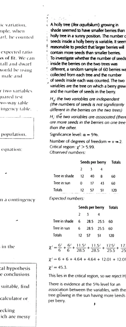
equation:

A holly tree (ilei

aquifolium)

growing

in

shade

seemed to have smafler berries than a

holly tree in a sunny position. The

number

of

seeds inside a holly berry

is variable, It

seems

reasonable to predict that larger berries hl

contain more seeds

than

smaller berties.

To investigate whether

the

number of seeds

inside the berries on the two trees was

different,

a

random

sample

of

60 berries was

collected from each tree and the number

of seeds inside each was counted. The two

variables are the tree

on

which

a

berry grew

and the number of seeds in the berry.

I1,:

the two

wjriob!es (JIC

independent

(the numbers of seeds

is

not significantly

different in the berries on the two trees)

II: th two variables ore associated (there

(Ire

more seeds in the berries on one tree

than the othe,

Significance level: a

=

5%

Number of degrees of freedom=

v

“2.

Critical region:

> 5,99.

Observed numbers:

(i-l)’

Seedsperberry

Totals

2

3

4

Tree in shade

12

40

8

60 Tree in sun

0

17

43

60 Totals

12

57

51

120 l:cli

expected

I

reqtiency

is

calculated

I

mm ‘a tieson a corn

i migt’ncy

Expected numbers:

table

using thus

equation:

_{Seedsperberry}

_Totals

row

total ><

column

total

2

3

4 grand total

_Treeinshade

₆

_28.5

_25.5

₆₀

Th ue

tin

tuber

I

degrees

ol

freedom

(v)

free in sun

6

28.5

25.5

60 Totals

12

57

51

120 where

in and a

are the

mirimher

til rmvs and coltttiins

in

the

_x

.Z

₊

I

Z+_!t_”

₊

_!Zz+

6

28.5

25.5

=

6

+

6

+

4.64

+4.64 ±

12.01

+

12.01

=453

This lies in the critical region, so we relect H

There is evidence at the

5°/o

level for an

association between the variables, with the

tree gi6wing in the sun having more eeds

per berry.

svlie me I

is I

lie ifiserved

I

req tiency

/

is t

lie

cx

petted

I

reqttencv a ml

is

the sum

ul.

tx

pect ed frequency

V = (in —

I

)(ii—

I

rout ingelicy

taNe.

The

chi-squared

test is just

one ol many

statistical hypothesis

tests. You must choose an

appropriate

one or

the

conclusions

that

you

ti raw may 111)1 he valid.

II the tests shown on the following pages aren’t suitable, find

out

about

others.

Most statistics calculations can he done using a calculator

or

spreadsheet.

Excel or other statistics software is

useful

for checking

calculations, or for statistics such as ANOVA which are messy

to

do with a calculator

(5)

4.’

Formost nvestigations, measures f the biologicalresponse are made From more than one sampling unit rho sample size (the

imher 1 _.arnplinq iii its) will vary iieperii nq on the resources iv uIthIn In ub 01 0 investigations 1111 simple ic iniy hi

ts small as twoor three (o_{q. two testtuhes in each treatment).}

o field tuities, each iiidividual may he u sampling mit, and the

‘ainple size can be very _{large (C g. 100 individuals), It is useful}

to summarize the data collected using descriptive statistics.

Variation in Data

Whether they are obtained from observation or experiments, most biological data show variability. In a set of data values, itis_{useful to know}

the value about which most of the data are grouped; the center value. This value can be the mean, median, or mode depending on the type of variable involved (see schematic below> The main purpose of these

sltistics is to summarize important trends in your data and to provide ibis basis br statistical analyses.

Descriptive statistics, such is neon, median,andmode, can help to highlight trends or patterns in thedata, Each of these statistics is appropriate to i;ertain types of data or distributions, e.g. a

mean is not_{appropriate tor data with a skewed distribution (see} below) Frequency graphs areuseful _{tor indicating the distribution} of_{d,rta Standard deviation and standard error are statistics used}

to quantify the amount of spread in the data and evaluate the reliability of estimatesof the true (population) mean.

Distribution of Data

Variability incontinuous data is often displayed as a frequency distribution, A frequency plot will indicate whether the dala have a normal disfribution (A), with a symmetrical spread of data about the mean, or whether the distribution is skewed (B), or bimodal (C). The shape of the distribution will determine which statistic (mean, mectian.nr _{node) best describes the central tendency} ofthe sample data

—

‘

ii r) ‘t S iO 3’ ‘5 ‘1 3 31 3546 O

Weight (g)

3)

ii I

‘‘ q

Oescriptive Statistics

Type of variable sampled

I

_I

Quantitative

(continuous or

discontinuous)

A: Normal distribution

Is

Ranked

-

Qualitative

I I

4

4 Mode

____

Mode

The shapeof the

distributionwhentIns

data are plotted

0

. Symmetrical — Skewed peak

or

_Two_peaks

peak

outliers present

(bimodal)

.

4

4 Mean

Median

Modes

Medlait

20 _{8: Skewed distribution}

z is

3)

10

U-20 _{C: Bimodal (two peaks)}

10

-J

0

‘

--

4

Mean Fbi’ average of ill dataentrres •Add up all the data entries

• Men uris ol. ntral tendency for

•Divide by the total number

iormafly distributed data

t ‘rita entries

Median • Fhe middlev _{tue when data} _{Arrange the data in}

entriOs Ireplacedin rink order incri’asinq_{rank order}

• A good rn asure ofentmai _{Identity the middle value}

I ndencv for skewed

tiUtributions • For an eren numberof

‘nines, find the mid Ooint

ofthe two middle values

Mode Themost commondatavolue .Identify the category with

• Suitable for bimodal distributions ‘he highest number of snd qualitative‘tata iata entriesi_{sing a tally}

h irt or bargraph

Range • Fins litference between the _{‘Fer’tify ‘he rn,3liest}

3’lij

m-iile t sod largest data values large I valu s 3ndtindthe . Providesacrude _{dication of} _{litforerw re}₁_{weerr then}

(6)

flormal distributIon

Measuring Spread

4raoqrain A haS a ,iandard ‘lei,ilion; he

iiuOS ,,ro spread wid&y

rroinid bra n,raafl,

0

rhestandard deviatIon is a trequentty used measureofthe variability (spread)

fl .1 Sot 0?data.It‘s usually prosentod

in the form * s. ri a normally

distributed set of data, 68% of all data

values wilt lie within one standard

deviation (s) of the mean ( and ¶15% of ill data values will tie within two standard deviations of the mean (left).

lioth plots show a normal distribution with a symmetrical spread of values about fho mean.

Calcutatlnq,

StandarddeviationiseaSity alculated usinq a

preadt’ierat,

rwo

different sets of datacanhwe the same mean and range, yet the

i’;tribotlon of data within the range can he quite different. In both the data se isicturad in the histograms below 68%

of_{the values li within the range i t}

s and ¶15% of the values lie within it

2s. However,in8, th data values are flora tightly clustered around the mean.

stflqram II has a -,rn.,iler siandard ievs,iion: Ito) vliira ire lustCri1 sore ighity iround hO mean.

Number o spcxes per frond

(in rank order

59 o6

‘30 ;6

¶11 ‘37

52 0

‘52 9

09 59

,3 70

03 ‘0 rmri

2. _{Calculate the mean, median, and mode of the data on beetle}

masses below. Draw up a tally chart and show all calculations: I ‘5

0

2.5%

.——

ii4. ,ts I

Site class

ci

I

.1

2 a

-a

U-0

25%

zH1

(Z *)

= sum of value * sum of value * sample size

.r.21 at.)s ,t,l, x.2g

11i

25%

Case Study: Fern Reproduction

Raw data (below) and descriptive statIstIcs (right) from a survey of the number of spores found on the fronds of a fern plant.

Raw data:

Number of spores per frond

64 60 64 62 68 66 63

69 70 63 70 70 63 62

71 69 59 70 66 61 70

67 64 63 64

TOtal of data entries

Numberofentries 25

Fern spores

Give a reason for the differences between the mean, median, md mode of the fern spore data:

‘2a i.) .r xii, x,2s

= 1641 = 68 spores

63 *‘.-.-.‘ 4

64 4

65 0

68 2

67 1

68

69 v’ ₂

‘b’ ₅

71 •‘

Beetle masses (q)

2.2 2.1 26

25 24 2.8