Figures of Speech in Strategic Communication
∗Sidartha Gordon†and Georg N¨oldeke‡
July 20, 2015
Abstract
We study a communication game in which the sender has a conflict of interest with the receiver, would prefer not to distort the truth, and is constrained by the inherent vague-ness of the language she shares with the receiver. In equilibrium, the trade-off is resolved in an endogenous truth-distorting figure of speech (exaggeration, understatement, irony), which the receiver interprets before choosing an action. There can be between one and five equilibria, unambiguously ranked in their informativeness. We characterize circumstances promoting the emergence and stability of particular figures of speech and obtain a number of comparative statics results. In particular, we find that a receiver may prefer a sender who is more dissimilar to him, less honest, or less competent. He may also prefer more vagueness in the language.
Key words: Strategic communication, Information transmission, Noise, Costly talk JEL Codes: C72, D82, D83
∗
We are grateful to audiences at University of Geneva, the Paris School of Economics, Sciences Po, University of Cergy-Pontoise, the Helsinki Center for Economic Research, Canadian Economic Theory Conference 2013 in Montreal, the Meetings of the Society of Economic Design 2013 in Lund, the Z¨urich-Basel Workshop in Micro Theory 2014, and the CIREQ Montreal Economic Theory Conference on the Economics of Persuasion and Communication for useful comments and suggestions. We are especially grateful to Mikko Mustonen for suggesting the hand clapping example, to Wei Li, Li Hao, Maxim Ivanov, Armin Schmutzler, Joel Sobel, Marko Tervi¨o, and Juuso V¨alim¨aki for comments and suggestions, and to Maria Goltsman for her discussion of the paper.
†
Department of Economics, Sciences Po, Paris, France, [email protected]. ‡
1
Introduction
Considerable attention has been devoted to studying situations where a Sender tries to influence the actions of a Receiver in a certain direction by communicating with him.1 An important characteristic of such situations in real life is that the Sender tends to use language in ways that exhibit certain patterns. A researcher applying for a grant might exaggerate how good his project is and how much money he will need to undertake it. A person writing a letter of recommendation may exaggerate how good he really thinks the candidate is, and perhaps understate his weaknesses. In both of these instances, if the Receiver understands the Sender’s behavior, he might be able to performs the rescaling that is needed to uncover the truth that is hidden in the words. In some cases, the Sender may resort to irony, using words whose literal meaning is the opposite of what he actually means and yet, be correctly interpreted by the Receiver. In this paper, we ask the following questions: (i) How is the truth distortion in the words spoken by the Sender linked with the conflict of interest? And (ii) how are these words linked to the amount of information that is transmitted in equilibrium?
In our model, the Sender and the Receiver share a natural language that one could interpret as a reference point, which is given by the literal meaning of the words, as found in the dictio-nary. We analyze relations between the three following objects. First, the conflict of interest. Second, the words the sender chooses, the way she chooses to speak. Third, the amount of infor-mation that is transmitted in equilibrium. Several papers in the abundant existing literature on strategic information transmission provide important insights on the relation between the con-flict of interest and information transmission but have relatively little to say about the choice of words (e.g. Crawford and Sobel, 1982). Others analyze the relation between the conflict and the words sent in equilibrium, but make extreme predictions on information transmission (Kartik, Ottaviani, and Squintani, 2007; Kartik, 2009; Chen, 2011), as they predict equilibria that are fully separating at least in some range of the type space. In the absence of noise, full separation implies that the Receiver can perfectly infer the truth behind any lie the Sender. Our contribution in this paper is to provide a framework that establishes links between these three objects.
One can think of many complicated ways in which people choose words. But there are recognizable patterns, some of which will be considered as lies and some of which will be con-sidered as mere figures of speech. It is remarkable that the same patterns are found in most languages and cultures, even though some cultures use some of these patterns more than oth-ers.2 Huebler (1983) writes “Attributing understatements to a predominantly English linguistic pattern of behavior is documented in many works dealing with the English way of life. Amongst such books are those aimed specifically at teaching English as a foreign language.” Our stylized model allows for three sorts of language distortions, or departures from the conventional literal meaning of words.
The first one, exaggeration or overstatement, is found in a variety of shades, from an outright lie to a simple figure of speech: a hyperbola. The second one, understatement, is also sometimes a lie and sometimes a rhetoric device: a litotes or a euphemism. Al Gore, former vice-president of the United States of America, has been for example accused of having
“exaggerated his past support for Roe v. Wade, [...] inflated his experience as a farmer, [...] overstated his Army service in Vietnam and understated his youthful experimentation with marijuana.”3
1
Starting with Crawford and Sobel (1982), see Sobel (2013) for a recent survey.
2For example, Anglo-English uses understatement more often than other European continental languages,
such as German (Wierzbicka, 2006).
3Shardt, Arlie, My Memo Said What? New York Times, February 16, 2000.
In what some consider Al Gore’s most famous exaggeration, he declared in March 1999 to the media
“During my service in the United States Congress I took the initiative in creating the Internet.”4
The third type language pattern that we consider is irony, defined as the use of words or messages with an intended meaning that is the opposite of their literal conventional meaning, as in the following example.
“Young Belarusians have adopted a novel strategy to protest their frustration at the humorless and iron-fisted regime of Alexander Lukashenko: they have started clapping. Organized by way of social media [...], the flash-mob rallies began last month as a peaceful means of working around draconian laws that prohibit unsanc-tioned public gatherings. At first, a few hundred met up in the capital’s Oktyabr Square and then fanned out into the city, breaking into spontaneous fits of clapping on sidewalks and street corners, much like sports fans celebrating a win on the way home. Their ranks have since swollen to several thousand. Lukashenko’s thugs, how-ever, saw nothing but a threat to public order. When scores of protesters assembled in downtown Minsk and regional centers Wednesday evening, as they have for five weeks running, police and plainclothes goons were waiting for them. Squads of men in tracksuits formed human chains to break up the gatherings, seizing everyone in their path. Many were punched or kicked on the ground before being dragged away into unmarked buses.”5
In our model, these patterns of exaggeration, understatement or irony, arise in equilibrium and resolve a trade-off between two forces: on the one hand the conflict of interest, i.e. the incentive for the Sender to mislead the Receiver, and on the other hand, some sort of prefer-ence of the Sender for certain messages, which also depends on his information. In our main formulation, following Kartik (2009) and Kartik, Ottaviani, and Squintani (2007), we assume that the Sender does not like to lie. More precisely, words have a literal meaning and absent the influence motive, the Sender would prefer to say the truth and to use this plain literal mean-ing. Therefore distortions from honesty and literal meaning occur only because of the strategic motive to manipulate the Receiver.
In an extension, following Chen (2011) and Kartik, Ottaviani, and Squintani (2007), we also consider a situation where the preference of the Sender for certain words arises endogenously because the Receiver is naive with some exogenous probability, meaning that he interprets the Sender’s words literally, without taking into account the Sender’s strategic incentive. This in turn causes the Sender to prefer certain messages.
Besides preferences over words, another important feature of our model is that we constrain the sender to use a vague language. People often use words that do not have a well-defined meaning, such as the words “critical” and “seriously” in
“The situation is critical. It should be taken very seriously.”
Following Shannon and Weaver (1949) and Blume and Board (2013), we model this noise as an additive component that is the same across all messages. While this may seem a strong assumption, it serves as an approximation for the fact that all words are vague to some extent. This assumption has the following important implication: an exaggeration, it is more informa-tive, in a Blackwell sense, than an understatement. The intuition is simple: when the Sender
4
Al Gore, March 19, 1999.
5
Jason Motlagh,Time, July 7, 2011.
exaggerates, a larger share of the message received is coming from the sender rather than from the noise. An exaggeration is more informative in the same way that an amplified sound is more audible in the presence of noise than the same noise when it is not amplified. It should be noted that unlike models where the Sender chooses the precision of his signal (Gentzkow and Kamenica, 2011, as in), in our model, the Sender does not consciously choose the precision of his signal. In particular, any given Sender type is unable to change the precision of the signal. All he can do is to mislead the Receiver. Informativeness arises as an endogenous equilibrium phenomenon, as in Crawford and Sobel (1982).
We find that equilibria always exist and that sometimes, multiple equilibria coexist, even in a restricted strategy space, the space of linear strategies. There can be up to five linear equilibria, all of them separating, yet only partially informative because the language is vague. There is always at least one, but at most three straight talking equilibria, in which both play-ers’ strategies are increasing. Exactly one of the following statements holds: either (i) there is exactly onetruthful orexaggerating equilibrium or (ii) there are between one and three under-stated equilibria. This result is important, as it indicates that there is never an indeterminacy on whether the Sender understates or exaggerates. We characterize the understatement and exaggeration regions in the parameter set. In addition to the straight-talking equilibria, there can also be up to two ironic equilibria, where both players’ strategies are decreasing.
We obtain several comparative statics result. We show that increasing the Sender’s sensitiv-ity to the state, i.e. how much he wants the receiver to react to the state, always increases the amount of information that is transmitted. This is the case even if the Sender is already more sensitive to the state than the Receiver. This result contrasts where Crawford and Sobel (1982), where increasing the conflict of interest always decreases the amount of information transmitted in equilibrium. We also obtain the surprising result that decreasing the lying cost may have the same effect. In both cases, the intuition is simple: a more sensitive Sender, or one who is less reluctant to lie exaggerates more in equilibrium, and this results in more information being transmitted.
In another result, we show that when the Sender is less sensitive than the Receiver, the level of language vagueness that is most preferred by the receiver is not zero. Again, the intuition is simple. Increasing vagueness commits the Receiver to react less to the Sender’s message, since it is mechanically less informative. This in turn results in the Sender exaggerating more and revealing more information in equilibrium. This increase in revealed information may compensate for the increased vagueness of the language, a finding that echoes results by Myerson (1991), Blume, Board, and Kawamura (2007) and Goltsman, H¨orner, Pavlov, and Squintani (2009) in models of noisy cheap talk. Last, we consider an extension where the Sender is not perfectly informed: he only observes a noisy signal of the state. We show that when the Sender is less sensitive to the state than the Receiver, it may be better for the receiver to listen to a less well informed speaker, a finding that echoes a result by Ivanov (2010) in the context of cheap talk communication. The intuition is similar as in the case of the noise increase. Hearing a Sender whom he knows is less informed commits the Receiver to react less to the Sender’s message. In equilibrium, the Sender may reveal more of his information. This increase in the information the Sender reveals may compensate the decrease in the quality of the information he possesses: the Sender knows less, but he says more.
1.1 Related literature
In addition to the papers already cited, our model is related to the literature on endogenous signaling, starting with Matthews and Mirman (1983) and Kyle (1985).6 In those models where firms or insiders signal private information through quantities or prices in the presence of noise,
6
the message (price or quantity) is also costly to the Sender in the sense that it enters his payoff through its profit function, but this type of cost is quite different than the one we consider here. The applications and interpretations of theses models are also very different from ours.
Our paper also contributes to the literature on pragmatics, which studies the question of how context contributes to meaning (Grice, 1975). In particular, in recent years, a growing literature has emerged that uses game theoretical models to address this question (Pinker, Nowak, and Lee, 2008; Mialon and Mialon, 2013; Blume and Board, 2013).
2
The Model
2.1 The Communication Game
There are two players, the sender and the receiver. The sender is privately informed about the state of the world θ ∈ Θ, which we often refer to as the sender’s type. After observing her type, the sender chooses a message m∈M. The message chosen by the sender determines the distribution of a signaly∈Y. The receiver observesy (but neither θ norm) and then chooses an action a∈A.
We assume that the type, message, signal, and action spaces are identical and given by Θ = M = A = Y =R. As in Kartik, Ottaviani, and Squintani (2007), the assumption that
the type and message spaces are identical affords the interpretation that the messagemhas the literal meaning that the state isθ=m and we adopt this interpretation throughout.
We assume that the receiver’s payoff is
UR(a, θ) =−(a−rθ)2 (1)
and that the sender’s payoff is
US(a, m, θ) =−(a−sθ)2−k(θ−m)2. (2)
The parameters r∈Rand s∈Rappearing in (1) and (2) describe the players’ most preferred
actions, which depend on the state and are given byrθfor the receiver andsθby the sender. For ease of exposition and without loss of generality we will assumes≥0 throughout the following.7 Following Kartik (2009), the real numberk >0 parametrizes the sender’s cost of lying, that is, sending a message with a literal meaning that deviates from her type. As we explain in Section 5.3 this cost need not arise from an intrinsic aversion to lying, but can be thought of as arising from the possibility that the receiver adopts a “naive” interpretation of the signal he observes. We do not impose any restrictions on r. Hence, our analysis allows for the possibility that, as far as the choice of optimal action is concerned, there is no conflict between the sender and the receiver (r=s), that the receiver is either more (r > s) or less (0< r < s) extreme than the sender, has opposing interests (r <0), or just doesn’t care (r = 0). These different cases have rather different implications for the structure of equilibria and we thus consider it important to consider them all.
To complete the description of our model, it remains to specify the distributional assump-tions. In a departure from what is common in the literature on communication games but in line with the literature on strategic information transmission in financial markets building on Kyle (1985), we assume thatθis normally distributed with zero expectation and varianceσθ>0 and
that the signalyobserved by the receiver is given byy=m+, whereis independent ofθand normally distributed with mean zero and varianceσ2
=vσ2θ >0. The parameter v >0, which
we refer to as the vagueness (of the language), measures the noisiness of the communication channel available to the sender.
7
2.2 Equilibrium
As it is standard for models in which the uncertainty faced by the players is described by normally distributed random variables, we restrict attention to equilibria in which the agents use linear strategies.8 A strategy for the sender is thus described by a parameterβ ∈R, where
m=βθ is the signal chosen by the sender if her type isθ. Similarly, a strategy for the receiver is described by the parameterλ, wherea=λyis the action chosen by the receiver if he observes the signaly. With the understanding that all strategies under consideration are linear, we refer toβ andλas strategies and to (β, λ) as a strategy profile.
Taking expectations in (1) and (2) we can write the player’s expected payoffs as functions of the strategy profile (β, λ) and the exogenous parameters:
uR(β, λ) =−
(λβ−r)2+λ2v
σθ2, (3)
uS(β, λ) =−
(λβ−s)2+λ2v+k(1−β)2σθ2. (4) Observing that σθ2 affects payoffs as a multiplicative constant only, we set σ2θ = 1 throughout the following and refer to a tuple (r, s, k, v) with s ≥ 0, k > 0, and v > 0 as a parameter constellation.
From (3), the unique best reply of the receiver to the strategy β of the sender is λ= Λ(β), where
Λ (β) = rβ
β2+v. (5)
From (4), the unique best reply of the sender to the strategy λ of the receiver is β = B(λ), where
B(λ) = k+sλ
k+λ2. (6)
Therefore the strategy profile (β, λ) is an equilibrium if and only if it solves the system
λ= rβ
β2+v
β = k+sλ
k+λ2.
(7)
2.3 Existence and Potential Multiplicity of Equilibria
We begin with two simple observations. First, from the equilibrium conditions in (7) it is immediate that for any parameter constellation withr = 0 there is a unique equilibrium given by (β, λ) = (1,0): If the receiver’s optimal action is always a= 0, he will chose that action no matter which signal he observes. As a consequence, the sender has no incentive to distort the truth and we thus obtain a truthful equilibrium with β = 1. Second, for any r it is optimal for the receiver to ignore the signal that he observes when β = 0, so that his unique best response isλ= 0. This in turn implies that truth-telling is the optimal strategy for the sender. Hence, due to the presence of lying costs, there never exists an uninformative equilibrium with
β = 0. Consequently, all equilibria in our model are separating, albeit – due to the vagueness of language – never fully revealing.
Substituting the first equation from (7) into the second and expanding the polynomial yields thatβ is an equilibrium strategy if and only if
kβ5−kβ4+2kv+r2−srβ3−2kvβ2+kv2−srvβ−kv2= 0. (8) 8In general, a pure strategy for the Sender is a functionµ: Θ→M, mapping types into messages, whereas a
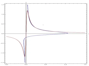
Figure 1: The best response functions Λ(β) of the receiver (plotted in red) and the best response functionB(λ) of the sender (plotted in blue) intersect twice in the negative orthant and thrice in the positive orthant, resulting in five equilibria. Parameter values are r = 0.076, s = 0.05,
k= 0.01 andv= 0.001.
Similarly, by substituting the second equation from (7) into the first, we obtain that λ is an equilibrium strategy if and only if
vλ5+ s2−rs+ 2kv
λ3+ (2ks−kr)λ2+ k2v+k2−krs
λ−k2r = 0. (9)
As the functions on the left side of these equations are polynomial of degree five and best responses are unique, it is immediate from the fundamental theorem of algebra that there exist at most five equilibria. Further, because the left side of (8) is strictly smaller than zero atβ= 0 and converges to +∞ for β → +∞, it follows that there exists at least one equilibrium with
β >0. Using Vieta’s formulas and Descartes’ rule of signs, we can refine these observations to obtain the following result. The proof of the statements in Proposition 1 that go beyond the ones we have already noted in the initial paragraph of this subsection are given in Appendix A.
Proposition 1. For all parameter constellations(r, s, k, v)there exists an equilibrium satisfying β > 0 and there exists no equilibrium satisfying β = 0. Moreover, if r = 0, then the unique equilibrium is (β, λ) = (1,0)and if r6= 0, then the following holds:
1. if r > 0 and s > 0, there exist at most three equilibria satisfying β > 0 and at most two equilibria satisfying β <0.
2. if r < 0 or s = 0, there exist at most three equilibria satisfy β > 0 and no equilibria satisfying β <0.
There are parameter constellations for which the upper bounds on the number of equilibria given in the statement of Proposition 1 are achieved. For the case r > 0 this is illustrated in Figure 1, which shows an examples in which the best response functions given in (5) and (6) have two intersections in the negative orthant and three intersections in the positive orthant. Note, in particular that for r > 0 there may indeed exists equilibria with β < 0. In such an equilibrium the messages used by the sender have the opposite of their literal meaning and we thus refer to such equilibria as ironic. In contrast, equilibria with β > 0 will be called
straight-talking.
2.4 A Change of Variables
For much of our subsequent analysis it is useful to rewrite the equilibrium conditions in (7) by introducing the parameter γ = λβ. This parameter measures how strongly the receiver’s response reacts to the underlying type of the sender and we thus refer to it as the reactivity. Multiplying both equations in the system (7) by β we can rewrite these equations as
γ =f(β)≡ rβ
2
v+β2 (10)
and
g(β, γ)≡kβ2+γ2−kβ−sγ= 0 (11) and identify equilibria with the solutions (β, γ) of equations (10)– (11) satisfying β 6= 0.9 In
the following we refer to (β, γ) withβ 6= 0 satisfying (10)– (11) as an equilibrium constellation. The corresponding equilibrium is given by (β, γ/β).
Equation (11) is equivalent to
β−1 2
2 q
k+s2
4k
2 +
γ−s
2
2 q
k+s2
4
2 = 1 (12)
and thus describes an ellipse with center (β, γ) = (1/2, s/2) and vertices (1/2, γ), (1/2, γ), (β, s/2), (β, s/2), where
γ = s 2 −
r
k+s2
4 , γ =
s
2+
r
k+s2
4 , β= 1 2−
r
k+s2
4k and β=
1 2 +
r
k+s2
4k .
For all β ∈
β, β, let γ1(β)≤γ2(β) be the two reals such that (β, γ1(β)) is the lower part
of the graph of the ellipse and (β, γ2(β)) is the upper part of the graph of the ellipse. More
precisely
γ1(β) =
s
2 −
r
s2
4 +k(β−β
2) (13)
γ2(β) =
s
2 +
r
s2
4 +k(β−β
2). (14)
Similarly, for all γ ∈[γ, γ] let β1(γ) ≤β2(γ) be the two reals such that (β1(γ), γ) is the left
part of the graph of the ellipse and (β2(γ), γ) is the right part of the graph of the ellipse. More
precisely:
β1(γ) =
1 2 −
r
1 4 +
sγ−γ2
k (15)
β2(γ) =
1 2 +
r
1 4 +
sγ−γ2
k . (16)
Observe that every equilibrium constellation (β, γ) must satisfy β ≤β ≤β and γ ≤γ ≤γ
as it corresponds to an intersection of the function (10) with the ellipse given by (11).
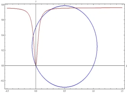
Figure 2 illustrates the determination of equilibrium constellations in (β, γ)-space as the intersections of (10)–(11). Observe that for any point on the graph of f(β) with β 6= 0, the best response Λ(β) of the receiver is equal to the slope of the line connection the origin to the point (β, f(β)). Similarly, the best responseB(λ) of the sender a to a strategy λis determined by the intersection of the line with slope λ through the origin and the ellipse given by the equation g(β, γ) = 0. In particular, the equilibrium value of λcorresponding to an equilibrium constellation (β, γ) is given by the slope of the line connecting the origin to the point (β, γ) in which (10)–(11) intersect.
9
Figure 2: Determination of equilibria as the intersections of the function f(β) describing the receiver’s best response (plotted in red) and the ellipse determined by the equationg(β, γ) = 0 describing the sender’s best response (plotted in blue). In this example there are again five equilibria. Parameter values are r= 0.76,s= 0.5,k= 0.9 and v= 0.002.
3
Uniqueness and Multiplicity of Equilibrium
As we have already established in Proposition 1, there always exists at least one straight-talking equilibrium. We may then think of the conditions for uniqueness of equilibrium as being of composed of two requirements. First, the absence of ironic equilibria and, second, the uniqueness of straight-talking equilibria. Contrariwise, multiplicity of equilibria may arise either because ironic equilibria exist or because there is more than one straight-talking equilibrium.
In the first of the following subsections we obtain necessary and sufficient conditions for the existence of ironic equilibria. Subsection 3.2 offers characterization results for straight-talking equilibria, including sufficient conditions for multiplicity and uniqueness of such equi-libria. Given the potential for multiple equilibria, it is of interest to inquire whether (and if so how) such equilibria can be ranked in terms of their informational content and their welfare implications for the sender and the receiver. Subsection 3.3 presents corresponding results.
3.1 Existence of Ironic Equilibria
As indicated by Proposition 1 ironic equilibria can only exist ifr >0 and s >0 hold, meaning that the sender and the receiver share a common interest to the extend that they both prefer actions to be increasing in the state of the world. It is intuitive that some communality of interest is required for irony to strive. Otherwise, if the receiver were to believe that the sender’s message signifies the opposite of its literal meaning, the sender would gain from switching to a straight-talking strategy thus confusing the receiver into taking an action more closely aligned to her true interests and saving on the lying cost associated with an ironic strategy.
While the parameter restrictions r >0 ands >0 are necessary for the existence of an ironic equilibrium, they are by no means sufficient.
Proposition 2. If kv−sr≤0 holds, then there exists no ironic equilibrium.
preclude the existence of a negative rood of the polynomial and, thus, the existence of an ironic equilibrium.
Proposition 2 implies that (given strictly positive values of the other parameters) sufficiently low values of k, resp. of v, are required for the existence of ironic equilibria. This is intuitive: language must be sufficiently precise to convey the irony intended by the sender and lying costs must be sufficiently small as otherwise the sender’s inherent preference for straight-talk will lead her to chooseβ >0 even if the receiver believes that the sender speaks with ironic intend. The fact that sufficiently high values of r and s are also required for the existence of ironic equilibria is less intuitive but makes sense in light of the consideration that for low values of
r the receiver’s reactivity will be low (undermining the sender’s incentive to bear the lying costs associated with using ironic language) and for low values of s the sender would prefer communication to be uninformative.
The following result shows that for strictly positive values of the other parameters, low k, lowv, highr, and highsare not only, as indicated by Proposition 2, necessary but also sufficient for the existence of ironic equilibria. The proof, which uses the alternative representation of the equilibrium conditions from Section 2.4, is in Appendix B.
Proposition 3. For all parameter constellations (r, s, k, v) with r > 0 and s > 0 there exists
¯
r >0, s >¯ 0, k >0, and v >0 such that two ironic equilibria exists if r >r¯, s > ¯s, k < k, or v < v holds.
3.2 Uniqueness and Multiplicity of Straight-Talking Equilibria
From Proposition 1 straight-talking equilibria exist for all parameter constellations and there are at most three of them. We have also seen that the upper bound of three straight-talking equilibria can indeed be achieved.
We begin by investigating what lies behind the multiplicity of straight-talking equilibria illustrated in Figure 2. Taking parameterssandkand, thus, the shape of the ellipse describing the sender’s best response as given, Figure 2 suggests that three conditions are sufficient to yield multiple straight-talking equilibria. First, f(β) should rise above the vertical intercept of γ2(β), which requires r > s. Second, f(β) should stay below the maximum of γ2(β), which
requires r < γ¯ = s/2 +√k+s2/2. Third, f(β) should attain values above s for values of β
sufficiently close to zero such as to generate the first intersection in the positive orthant visible in Figure 2. This last condition will be satisfied for sufficiently small values ofv. The proof of the following proposition, given in Appendix C, confirms that this intuition is correct and can be applied analogously to yield a sufficient condition for the existence of multiple straight-talking equilibria when interests are opposed.
Proposition 4. Suppose
s < r < s
2 + √
s2+k
2 (17)
or
s
2 − √
s2+k
2 < r <0 (18)
holds. Then there existsv >0 such that for parameter constellations(r, s, k, v) withv < v three straight-talking equilibria exist.
that, even though the equilibrium values of β may be quite different, in all three equilibria the responsiveness γ is close to both r and s, indicating that in each of the equilibria the actions chosen by the receiver are close to both player’s optimal actions. Condition (18) is in the same spirit as condition (17) in the sense that the first inequality indicates that the absolute difference between r and s must be small. However, here the second inequality does not simply require thatr is smaller thans, but (in cases >0) requiresr to have the opposite sign. We note that both conditions (17) and (18) are applicable in the case s= 0, so that multiple equilibria may exist even when the sender’s optimal action is independent of her type.
The following result establishes that, as suggested by the conditions in Proposition 4, mul-tiple straight-taking equilibria can only arise if the receiver is more extreme than the sender or has opposing interests. Further, if there are multiple straight-talking equilibria they are all
understated in the sense that in every equilibrium 0< β <1 holds. The proof is in Appendix D.
Proposition 5. For all parameter constellations (r, s, k, v) the following holds:
1. ifr = (1 +v)s, then there exists a unique straight-talking equilibrium and this equilibrium satisfiesβ = 1.
2. if 0 < r < (1 +v)s, then there exists a unique straight-talking equilibrium and this equi-librium satisfies β >1.
3. if r <0 or r >(1 +v)s, then all straight-talking equilibria satisfy 0< β <1.
To see the intuition for this result, consider, first, the caser=s(1 +v). In such a parameter constellation, the best response of the receiver toβ= 1 is to choseλ=s, so that conditional onθ
the receiver’s expected action is the one the sender wants him to choose, namelyγθ=sθ. Hence, there is no incentive for the sender to distort her message from the truth and (β, λ) = (1, s) is an equilibrium. As indicated by (10) if the sender were to choose 0 ≤ β <1, the resulting reactivity would be lower than s, providing the sender with an incentive to increase β, both to achieve a better alignment of the receiver’s expected response with her own interests and to save on lying costs. Similarly, if the sender were to chooseβ >1, the resulting reactivity would be higher than s, providing the sender with an incentive to decrease β. Consequently, in this case there is a unique straight-talking equilibrium, which istruthful, that is, satisfies β= 1.
Using similar arguments, it is easy to see that every straight-talking equilibrium for a pa-rameter constellation with r < s(1 +v) must be exaggerated, that is, satisfy β > 1. What is less clear is that the uniqueness result also obtains in this case. In particular, whenf(β)< s/2 holds, equilibrium occurs on the lower, increasing part of the ellipse inβ-γ-space. Here not only does the receiver’s best response to an increase inβ lead to an increase in the reactivity, but an increase in reactivity in turn provides the sender with an incentive to increase β, thus setting the stage for the co-existence of multiple equilibria. The main complication in the proof of Proposition 5.2 is to show that, despite this complication, straight-talking equilibrium is unique in this case. We note that Proposition 5.2 covers the case r =s in which sender and receiver agree about the optimal action. Here the equilibrium is exaggerated rather than truthful be-cause the vagueness of the language biases the receiver’s response towards zero, thus inducing the sender to speak more loudly to improve the informational content of the receiver’s signal, even though doing so imposes a cost of lying on the sender.
It is an immediate implication of Proposition 5 that either r < 0 or s < r must hold for multiple straight-talking equilibria to exist. Hence, it is clear that the corresponding inequalities appearing in the sufficient conditions for the existence of multiple straight-talking equilibria in Proposition 5 cannot be relaxed. While the same is not true of the other two inequalities appearing in (17) and (18), the first part of the following proposition establishes that multiplying the bounds appearing in these inequalities by 2 provides a simple necessary condition for the existence of multiple straight-talking equilibria, thus establishing that when the interests of the sender and the receiver are sufficiently divergent, uniqueness of straight-talking equilibrium is assured. Similarly, the second part of the following proposition shows that v ≥1/4 implies uniqueness of straight-talking equilibrium, so that – as suggested by the statement of Proposition 5 – multiple straight-talking equilibria can only arise when language is sufficiently precise. Finally, we also consider the role of the communication cost parameterk for the uniqueness of straight-talking equilibria in the case, establishing that when lying costs are either sufficiently high or sufficiently low such uniqueness is assured. The proof of the following is in Appendix E, which also provides the definitions of the functions k(r, s, v) and k(r, s, v) appearing in the statement of the third part.
Proposition 6. The following conditions are sufficient for the existence of a unique straight-talking equilibrium:
1. r≥s+√s2+k or r≤s−√s2+k holds.
2. v≥1/4 holds.
3. k≥k(r, s, v) or k≤k(r, s, v), where k(r, s, v)>0 holds for all(r, s, v).
The intuition for Proposition 6.3 is the following. When lying costs are sufficiently high, the sender will not stray far from truth-telling in equilibrium, so that in any equilibriumβ must be close to 1. Multiplicity of straight-talking equilibrium, however, is only possible if there exists an equilibrium with 0 < β < 1/2, cf. Figure 2. Vice versa, recalling from our discussion of Proposition 5 that the possibility of multiple straight-talking equilibria only arises in cases in which the sender has an incentive to understate her type, when lying costs are sufficiently low in every straight-talking equilibrium β must be close to zero, precluding the possibility of the existence of an equilibrium withβ >1/2.
3.3 Informational Content and Welfare across Equilibria
A standard question in models such as ours is “How much information is transmitted in equi-librium?” In a model with normally distributed random variables it is natural to measure “how much information” by considering the ratio of the precisions of the receiver’s posterior (after having observed the message) and prior (before having observed the message) forecast of θ. The prior precision is 1/σ2
θ. The posterior precision after having observed the signal βθ+
is 1/σθ2+β2/σ2 (this uses standard formulas for the precision of normally distributed random variables). Hence, the ratio of the precisions when the sender uses the strategy β is simply
π(β) = 1 +β2/v. (19)
The following result follows directly from the definitions.
Looking at the picture, I see that the following is correct, but the claim that the ironic equilibria have lowerβ2than the straight-talking equilibria requires proof.
Multiplying both sides of the equation for the receiver’s best response by λand using the definition γ = λβ we obtain that for any profile (β, λ) on the receiver’s best response, the relation
λ2v= (r−γ)γ (20)
holds. Substituting this into the formulas for player’s expected utilities given in (3) and (4) and recalling our normalizationσ2θ = 0 we obtain (with slight abuse of notation):
Lemma 1. Let (β, γ) be an equilibrium constellation. Then the corresponding equilibrium utilities are given by
uR(β, γ) =−r(r−γ)
uS(β, γ) =−
(γ−s)2+ (r−γ)γ) +k(1−β)2.
Using these expressions, one can immediately rank the equilibria, from the point of view of the receiver’s welfare. This is because in any equilibrium, γ ≤r holds and uR is increasing in
γ.Therefore the receiver prefers the equilibrium which has the highest value ofγ, which is also the most informative one. This gives the following result.
The above is written under the presumption thatr >0 holds. We want to rephrase so that the caser <0 is covered, too. (For instance, by preceding the current argument with saying that it is aboutr >0 and then noting thereafter that an analogous argument applies to
r <0. We also want to add a sentence of explanation reminding the reader that in equilibrium there is a one-to-one relationship between
β2andγ.
The current statement of the following result is very clumsy. We want to make sure that the essential point is easily grasped – the re-ceiver always likes the loudest straight-talking equilibrium best. (I don’t see why we or anyone else should be much interested in the rank-ing of the other equilibria – except that it is noteworthy that the receiver really doesn’t like irony.)
Proposition 8. If these equilibria exist, the receiver ranks equilibria as follows. The gentle ironic is the worst (if there is any), followed by the loud ironic (if there is any), followed by the gentle straight talking (if there is any), followed by the middle straight talking (if there is any), followed by the loudest equilibrium, which is the receiver’s preferred equilibrium.
The sender’s utility over pairs (β, γ) on the receiver’s best response curve is given by
(2s−r)γ −k(1−β)2.
I am not sure were the conclusion that the straight-talking equilibrium is preferred in the following paragraph is coming from. I see there is an argument, but I don’t get it. (It might help to not talk about arbitrary points on the best-reponse curve but to start out by saying that straight-talking equilibrium is unique and then asking how it compares to an ironic one. I think it would also be useful to tell/remind the reader what the condition 2s > rmeans in terms of the figure. There is no reason to mention at the end that we can-not rank the ironic ones. What we and the reader should care about that in this case the sender and the receiver agree on what the best equilibrium is.
If 2s > r, this implies that the sender’s ideal point (β◦, γ◦) on the receiver’s best response curve is such that β◦ > 1. In this case, the sender’s utility is single-peaked in β for positive values of β. Moreover, between two points (β, γ) and (−β0, γ0),with 0 < β0 ≤ β ≤ 1, on the receiver’s best response curve,the sender prefers the first. In other words, if an ironic pair is preferred to a straight talking one, the former must be louder. But when 2s > r, we know that there is a unique straight talking equilibrium and either no or two ironic equilibria. In this case, it is clear that the unique straight talking equilibrium is preferred to the two ironic equilibria, if they exist. How the sender ranks the two ironic equilibria is not immediately clear.
I don’t get the case distinction at the beginning of the following paragraph – we can have bothr >2sandr < s, can’t we? In any case: It seems to me that we want to (a) focus on the question what the BEST equilibrium from the perspective of the sender is. If the upshot here is that we cannot say very much, then we shouldn’t spend much time on this. If we have some simple conditions under which the sender also likes the loudest one best – state them. Other than that I think what we really want to do is to give an example (i) in which the sender prefers a straight-talking equilibrium which is not the loudest one and – if possible – (ii) one in which the sender likes an ironic one best. (If we know that the latter can’t happen, we should state that – I can’t see why this should be true. Whatever example we give, we should offer some intuitive discussion to explain what is going on.
If r > 2s, this implies that the sender’s ideal point is (1,0),while if r < s, his ideal point is (1,+∞). In both cases, it is not immediately clear how the sender ranks equilibria. In the second case, if the loudest equilibrium is understated (or if it does not exaggerate too much),
4
Comparative statics
It would be nice to have a more eloquent title for this. There is a sense in which all the results we have obtained so far are purely techni-cal ones - they are interesting only to the extend that our model is considered to be interesting. In most cases, however, a model is only considered interesting if it yields interesting substantive results. So, this section should be about substantive results, which (we hope) we can sell in the introduction and which convince the reader that our model is interesting!
In this section, we establish comparative statics results on equilibria and welfare. We study changes in the sender’s sensitivitys,in the lying costk,and in the vagueness of the languagev.
4.1 Changing the sender’s sensitivity
Needs to have a motivating paragraph – what are the interesting issues one might wonder about here? I don’t think it makes much sense to put equal weight on the comparative statics of all equilibria. I propose to focus on the loudest straight-talking one – we can justify this to some degree by the receiver’s preference for it – and talk about the other equilibria only to the extend that something interesting and/or unexpected happens to them.
The effect of increasing sis easy to understand in terms of the (β, γ) diagram. We keep the points (0,0) and (1,0) fixed and “stretch” the ellipse by pulling at the points (0, s) and (1, s) in the vertical direction. Consequently, the effect will be the following:
• r > 0, straight talking either exaggerated or slightly understated equilibrim, or any strongly understated equilibrium that is not the middle one: bothβ andγ increase.
• r > 0, straight talking, strongly understated equilibrium in the middle: both β and γ
decrease.
• r >0,ironic equilibria: Starting from a situation in which no ironic equilibria exist (for low
s), at some point an ironic equilibrium appears and splits into two ironic equilibria. The one with the greatest absolute value of β moves towards an even higher β (in absolute value) and a higher value of γ. The other one moves towards the origin, i.e. a lower absolute value ofβ and a lowerγ.
• r <0 : if there is a unique one, it moves towards the origin, i.e. a lowerβ and also a lower
γ in absolute value.
4.2 Changing the cost of lying
Needs to have a motivating paragraph – what are the interesting issues one might wonder about here? I don’t think it makes much sense to put equal weight on the comparative statics of all equilibria. I propose to focus on the loudest straight-talking one – we can justify this to some degree by the receiver’s preference for it – and talk about the other equilibria only to the extend that something interesting and/or unexpected happens to them.
The effect of increasingkis easy to understand by thinking in terms of the (β.γ) diagram. We keep the points (0,0),(s,0), (1,0),(1, s) fixed and “stretch” the ellipse by pulling at the points (1/2, γ) and (1/2, γ) in the vertical direction. Consequently, the effect will be the following:
• r >0, straight talking, exaggerated equilibria: β andγ fall as k increases.
• r > 0, ironic equilibria: Starting from a situation in which two of these exists, the one with the greatest absolute value ofβ moves closer to the origin askincreases and the one with the smallest absolute value ofβ will move in the opposite direction until they both merge and disappear.
• r < 0: if there is a unique one β and the absolute value of γ increase as k increases. Multiplicity story is akin to the one for the r >0 case.
An interesting implication of these results and the ones obtained in the previous section is the fact that when 0< r < s(1 +v) the receiver’s equilibrium utility is actually decreasing ink. One might have thought that it is always to the receiver’s advantage if the sender’s incentive to mislead him is reduced.
The following is a nice result and we should emphasize it (and avoid saying that the intuition is simple...)
Proposition 9. Suppose that 0< r < s(1 +v) holds. Then the informational content and the receiver’s expected utility are decreasing in k at the (unique) exaggerating equilibrium.
The intuition of this result is simple. As moral norms against lying becomes weaker, the equilibrium involves more exaggeration. In equilibrium, information is encoded in a more exag-gerated language, which implies a better transmission of information, as the relative importance of the noise decreases, due to how “loud” the sender speaks.
I think we should move the following limit cases to a separate discussion section. The point of these is to understand how our model re-lates to simpler models that one might have thought of and this is exactly the kind of thing that a discussion section is good for.
4.2.1 Limit as k→ ∞
It is not clear why we want to worry about this limit at all. We should only keep this, if we are able to come up with an introductory paragraph motivating why this is an interesting limit to consider. I can’t think of such a paragraph.
For large enough k we have a unique equilibrium (βk, γk) satisfying βk → 1 and γk →
r/(1 +v).
In terms of the welfare analysis it is not immediately obvious whether the term k(1−β)2 converges to zero. However, using (11) we know that
k(1−β)2= (γ−s)γ
1
β −1
(21)
holds in every equilibrium. Asβ →1 andγ has a finite limit, it follows thatk(1−β)2 converges to zero as kconverges to infinity.
uS =−
(r−s)2+s2v
1 +v σ
2
θ+ (c−b)2 anduR=−
r2v
1 +vσ
2
θ
(One should check whether the above is what one gets “in the limit”, that is, by simply presuming that the sender is an automaton who has to tell the truth. I think it should. That would help in clarifying that the remaining costs result from the fact that (a) the seller gets his way in expectation with (b) the noisiness of the communication channel imposing an additional cost hurting both players.)
4.2.2 Limit as k→0
Before starting out on this, we want to explain what happens in a model in whichkis simply set to 0. This sets the state for asking the question whether these equilibria “at the limit” coincide with the limit set of equilibria whenk→0. From what is written below, it is not clear to me what the answer to that question is. But it is the question that we want to focus on. Other than that we simply want to note when something unexpected happens and explain the intuition for it.
For r > 0 and sufficiently small k there are exactly three equilibria, two ironic ones and a straight talking equilibrium. The gentler (unstable) ironic equilibrium converges to (β, λ) = (0,0),which is the babbling equilibrium. (As none of the other equilibria converges to babbling this establishes a sense in which the babbling equilibrium – that always exists whenk= 0 – is not stable.)
For the loud ironic and the straight talking equilibria, there are two cases to consider: s≥r
and s < r.
• r≤s.In this case, the sequence of straight talking equilibria (βk, r) converges to (+∞, r)
and the sequence of load ironic equilibria converges to (−∞, r).In either case, the infor-mational content of equilibrium goes to infinity and the equilibrium utility of the receiver converges to 0 – which is the receiver’s ideal outcome. Understanding what happens to the sender’s payoff is a bit more challenging. Suppose, first, that b=c holds, so we can ignore the last term in the sender’s payoff. Using (21) and β → ∞, γ → r, we find that the termk(1−β)2 converges to (s−r)r – hence, unless r=sthe expected lying costs to be borne by the sender do not converge to zero. The sender’s utility converges to (s−r)r.
10 Now, let’s assume b6=c. The question then is what happens to the term (r−γ)r/kv
ask converges to zero. This is not obvious as r−γ and k both go to zero, so we might want to take a closer look at (r−γ)/k. In fact, rather than doing that let us return to the expression λ2/k as the one describing the expected cost of “lying about the intercept.” This term can be rewritten 11 as
λ2 k =
β−1
β γ
s−γ. (22)
As β goes to infinity, the first fraction goes to 1, demonstrating that in the case r < a
we get a strictly positive limit given by r/(s−r). (I find it somewhat puzzling that this expression is strictly increasing in r.) In the special case s = r we get that the cost converges to infinity. (So if there is only conflict about the intercept the costs go off to infinity. If, however, there is an additional conflict about slope that this effect gets tempered - providedr < s holds.)
• r > s.In this case, the two equilibrium values ofβ converges to the positive and negative solution of
s r =
β∗2
β∗2+v,
i.e.
β∗ =±
r v
1−r s
and γ∗ =s.
Observe the limit of the straight talking equilibrium can be gentle, loud, truthful, or exaggerated depending on how the value of the ratior/s, e.g. r =s(1 +v) implies β∗= 1 etc. (the case distinction is exactly in line with what we have seen before).
Observe: In the case b = c there are no lying costs in the limit and in expectation the sender gets his most preferred action. Nevertheless, the sender does not obtain his bliss utility as λ converges to a finite limit, implying that the noise cost-term λ2v does not vanish in the limit, but converges to (r−s)s >0. Ifb6=cit is clear from the calculations that we did above and the fact thatβ cannot converge to 1 that the expected cost of lying about the intercept go to infinity.
10Observe that keepingsfixed this term is maximized forr=s/2. This is consistent with the highest possible
amount of exaggeration occurs whenf(β) =s/2.
11
4.3 Changing the vagueness of the language
I believe we want to focus on the comparative statics of the loudest straight-talking equilibrium here. Other observations should be rele-gated to footnotes and or remarks. Of course, it would be good if we could point to anything unexpected, non-obvious happening here.
Increasing v flattens the function f.
Consider straight talking equilibria for r > 0 and suppose equilibrium is unique. The equilibrium value ofβ will then be increasing inv until we hit the point at whichf(β) =s/2. Thereafter the equilibrium value of β is decreasing and converges to 1 as v → ∞. If v is sufficiently small (and r sufficiently large) that β < 1/2 holds for small enough v, then the equilibrium value of γ will first be increasing in v and then – once β = 1/2 has been hit – decreasing inv.
Considering the ironic equilibria for r > 0,it is clear that these will cease to exist for v
sufficiently large. As long as they exist, the gentle (unstable) one will move away from babbling when v increases, whereas the comparative statics of the louder ironic equilibrium (I am again taking it for granted that there are at most two ironic equilibria) are determined by whether equilibrium sits onγ2 orγ1. If it sits onγ2, then the absolute value ofβ is increasing inv until
it reaches β = β is reached; thereafter we move on γ1 with β decreasing until we bump into
the unstable equilibrium and both disappear. Throughout γ is decreasing in v for the stable equilibrium.
Consider the caser <0 under the additional assumption that we have uniqueness. Then β
is increasing inv and γ is decreasing inv forβ <1/2 and increasing thereafter.
4.3.1 Limiting behavior of all equilibria when the language vagueness is low
This should, I believe be moved to the discussion section, too. Again, it should be motivated by some question before we start dwelling on the results.
Let r >0.
Keeping all other parameters fixed, in the limit where v goes to 0 :
• If
r s ≤1,
there is a unique positive equilibrium, that converges to (β2(r), r), i.e. β = β2(r) and
λ= βr
2(r).There are also two negative equilibria. One that converges to (0,0),i.e. β= 0 and λ=−k
s, and another one that converges to (β1(r), r),i.e. β =β1(r) and λ= r β1(r). • If
1< r s <
1 2 +
q
k s2 + 1
2 ,
there are three positive equilibria. Two of them converge respectively to (β1(r), r) and
to (β2(r), r).The third one converges to (0, s), i.e. β = 0 andλ= +∞. There are also
two negative equilibria. One that converges to (0,0),i.e. β = 0 andλ=−k
s, and another
one that converges to (0, s),i.e. β = 0 and λ=−∞.
• If
1 2 +
q
k s2 + 1
2 <
r s,
there is again a unique positive equilibrium that converges to (0, s), i.e. β = 0 and
4.3.2 Optimal vagueness
We certainly want to keep this and sell it as well as we can.
Noise has a direct negative on the welfare of both players. It has also an indirect strategic effect. For positive (negative) equilibria that lie on some increasing (decreasing) portion of the ellipse, a noise increase has a positive effect on the receiver. The opposite is true for equilibria that lie on some decreasing (increasing) portion of the ellipse.
The welfare effect on the sender is more complex, because the lying cost also plays a role. Assume r >0 and focus on straight talking equilibria.
If r ≤s(so that the unique straight talking equilibrium is always exaggerating) it is clear that the receiver prefers noise to be as small as possible and in the limit for v→0 obtains his bliss point with γ=r.
If r > sthe question of the optimal noise level is more interesting (and we have to grapple with the problem that there might be multiple equilibria).
In particular, when s < r < s/2 +√s2+k/2 we have already seen that there are two
equilibria such that the receiver obtains his bliss point in the limit asv→0. There is, however, also a third equilibrium in which γ converges tos. So there is a risk that the receiver may end up in the “wrong” equilibrium.
If r is greater than the upper bound just given, pushing v to zero is not what the receiver wants to do. Rather he wants to choose v such that equilibrium occurs at β = 1/2 – which is the best the receiver can hope for. It is not immediately obvious to me, though, that this equilibrium must then be unique. If it is not, the same question as in the previous case arise. This is summarized in the following result.
Proposition 10. Suppose that r > γ.The informational content and the expected utility of the receiver are both increasing in v in 0,r4−γγi and decreasing inv onhr4−γγ,+∞.
5
Extensions
In this section we consider three extensions of the model. In the first one, we consider different preferences over actions that include a constant term in the sender’s bias. In the second one, we drop the assumption that the receiver perfectly observes θ. In the third, we study a model where the sender does not have a lying cost, but where the receiver can be naive with some probability. We show that this alternative model can be mapped to our model.
5.1 Constant sender’s bias
I don’t think this extension adds a lot of value. If you think this is exciting, you might want to try to convey better why this is so. If this is only here because other people have had such a bias in their models, you might consider giving this as the last extension or, possibly, move it to the appendix.
In this section, we assume that the Receiver’s payoff is
UR(a, θ) =−(a−[rθ+b])2,
and that the Sender’s payoff is
US(a, θ) =−(a−[sθ+c])2−k(θ−m)2.
The parametersb,c,r and sare real numbers. As before, without loss of generality we assume
s≥0. We look for equilibria in which players use “linear” strategies.
µ(θ) =βθ+µ0
The unique best reply of the receiver to a linear strategy (β, µ0) of the sender is linear with
parameters (λ, α0) satisfying
λ=r β
β2+v and α0 =b−λµ0. (23)
These equations follow upon observing that the receiver’s best response is given by rE[θ |
y] +band that from the linear conditional expectation property of normally distributed random variables we haveE[θ|y] = β2β+v(y−µ0). The second equality has the following interpretation.
The expected message sent induces the expected preferred action of the receiver. The unique best reply of the sender to a linear strategy (λ, α0) of the receiver is linear with parameters
(β, µ0) satisfying
β = k+sλ
k+λ2 and µ0=λ
c−α0
k+λ2. (24)
These equations follow from substitutinga=λ(m+) +α0 into the expression for the sender’s
payoff, taking expectations with respect toand then maximizing with respect tom.
If (β, λ) solves the system 7, which is equivalent to (β, λ) being an equilibrium of the model analyzed in Sections 2 and 3, then the system
α0 =b−λµ0
µ0 =λcλ−2+αk0.
has a unique solution given by
µ0=
λ
k(c−b) andα0 =b− λ2
k (c−b). (25)
Therefore the problem of finding equilibria can be reduced to the problem of finding the solutions (β, λ) to the system (7). Furthermore, taking the solution to (25) into account, we can we can write the player’s expected payoffs as functions of (β, λ) and the exogenous parameters:
uS(β, λ) =−
(λβ−s)2+λ2v+k(1−β)2
σθ2−k+λ
2
k (c−b)
2. (26)
uR(β, λ) =−
(λβ−r)2+λ2vσθ2. (27)
Setting b = 0, and c > 0, we obtain the following interesting comparative statics results on changes in c.
Proposition 11. Let b= 0 and c >0.An increase inc has no effect on the equilibrium values of λ and β.The equilibrium values ofα0 decrease. The equilibrium values of µ0 increase if the
equilibrium is straight-talking (λ > 0)and decrease if the equilibrium is ironic (λ <0). Such a change has no impact on the welfare of the receiver in each of the (possibly many) equilibria. It decreases the welfare of the sender.
5.2 The sender’s competence
I like this one and think we should keep it.
Suppose then that the sender does not perfectly observe θ, but only θ+δ, where δ is a normally distributed random variable with mean 0 and variance σ2
δ. We assume that the
variables θ, δ and εare independent. It is convenient to define
w= σ
2
δ
σ2
θ
.
Note that the case w = 0 coincides with the main model: it is the case where the sender is perfectly informed onθ.As in the main model, we look for equilibria where the sender sends a message equal toβ(θ+δ) and the receiver takes an action equal toλy.One can show that the best response of the receiver is
λ= rβ
v+β2(1 +w)
while the best response of the sender is
β= k+
s
1+wλ
k+λ2 .
This model can be mapped in our main model as follows. Consider the change of variable
s0= s 1 +w; r
0 = r
1 +w; v
0 = v
1 +w andk 0 =k.
We have the following result.
Proposition 12. The profile (β, λ)is an equilibrium of the game with an imperfectly competent sender with parameters s, r, v, k and w if and only if the same profile (β, λ) is an equilibrium in the main model, with parameters s0, r0, v0 and k0.
We are interested in the effect of a decrease in the sender’s competence (i.e. an increase in
w) on the equilibrium strategies and on the receiver’s welfare. An increase in w affects both the best-responses of the receiver and of the sender: it decreases both of them. In the case of a straight-talking equilibrium that is either exaggerated, truth-telling or slightly understated, these effects work in the same direction: they decrease the equilibrium value of γ = βλ and therefore decrease the receiver’s welfare. This result is expected: the sender is less informed and this decrease in information is passed on to the receiver. In the case of a strongly understated equilibrium, the effects work in opposite directions. The decrease of the best response of the receiver tends to increase γ, while the decrease of the best response of the sender tends to decrease γ.The magnitude of the later effect is turned-off whens= 0 and is dominated by the former whensis small. Thus we obtain the following result.
Proposition 13. When s is small enough and the equilibrium is straight-talking and strongly understated, a decrease of the sender’s competence increases the welfare of the receiver.
5.3 Naive receivers
We want to do at most one of the following two cases in the main body of the paper. We could then note that one might to want model things differently and cover the other case in the appendix.
We now consider an alternative source of preferences over specific words. Even if the sender does not have psychological costs of lying and maximizes only the expectation of the utility he derives from the receiver’s action, that is−(a−sθ)2, the receiver could be naive with positive probabilityκ∈(0,1) and strategic with probability 1−κ. A naive receiver interprets messages literally, without taking into account strategic incentives of the sender. This is because he believes that the sender is reporting his type in a truthful manner. This behavior in turn creates an endogenous message cost for the sender. Similar behavioral types were studied by Chen (2011), in a game of communication without exogenous noise. We will show that in our context, this model is in a certain sense equivalent to ours. This means that in our model, the lying costkneed not be taken literally, as it can arise endogenously from the possibility in the sender’s mind that the receiver may be naive.
We distinguish two cases, depending on whether or not the naive receive is aware that the message sent by the sender is subject to noise. In either case a naive receiver has the same preferences as a rational one, he maximizes the expected value of his utility −(a−rθ)2. A rational and a naive receiver only differ in their belief overθ.As in the main model, given that the sender sends message βθ when his type is θ, the best response of a rational receiver is to choose actionλy,with
λ= rβ
v+β2. (28)
5.3.1 The naive receiver is also unaware of the noise
We consider here the case where the naive receiver is also unaware of the noise. Upon receiving the garbled messagey, the naive receiver believes that the sender’s type is y. He thus chooses actionry. Given that the sender expects the receiver to take action ry with probabilityκ and
λy with probability 1−κ,he maximizes
Eε
h
−(1−κ) (λ(m+ε)−sθ)2−κ(r(m+ε)−sθ)2|θi
which is maximized by sending the message m=βy such that
β =
κ
1−κ
r2+rλ
κ
1−κ
r2+λ2
s
r. (29)
Consider the following change of variable:
e
β =βr
s; eλ=λ; er=
r2
s; ev=
vr2
s2 ; es=r andek=
κ
1−κr
2.
Then (β, λ) solves the system (28)(29) if and only ifβ,e eλ
is a solution of the system (7) with
parameters r,e ev, esand ek, i.e. if and only if it is an equilibrium in our main model with those
parameters. It is now clear that this model maps to our main model in the sense made clear by the following proposition.
Proposition 14. Let (β, λ) be an equilibrium of of the game without lying cost, where the receiver is possibly naive and unaware of the noise with parameters r, s, v and κ. Thenβ,e eλ
is an equilibrium in the main model with parameters er, ev, esand ek.
5.3.2 The naive receiver is aware of the noise
We now turn to the more complicated case where the naive receiver is aware of the noise. Upon receiving the garbled message y, the naive receiver only differs from a rational one in that he believes that the sender is truthful, i.e. plays β = 1. This implies that his optimal action is
r∗y, with r∗ = v+1r , instead of ry in the version of the model where the naive receiver is also unaware of the noise.The rest of the analysis is identical in the two versions of the models. We obtain the best response functions:
λ = v+rββ2
β = (
κ
1−κ)( r
1+v)
2
+( r
1+v)λ
( κ
1−κ)( r
1+v)
2
+λ2
s(1+v)
r .
(30)
Consider the following change of variable:
b
β =β r
s(1 +v); bλ=λ; br=
r2
s(1 +v); bv=
vr2
s2(1 +v)2; sb=
r
1 +v andbk= κ
1−κ
r
1 +v
2
.
Then (β, λ) solves the system (30) if and only if
b
β,bλ
is a solution of the system (7) with
parameters r,b bv, bsand bk, i.e. if and only if it is an equilibrium in our main model with those
parameters. It is now clear that this model maps to our main model in the sense made clear by the following proposition.
Proposition 15. Let (β, λ) be an equilibrium of of the game without lying cost, where the receiver is possibly naive but aware of the noise with parameters r, s, v and κ. Then
b
β,bλ
is an equilibrium in the main model with parameters br, v,b sband bk.
In particular, it is clear that increasing the probability that the receiver is naive is equivalent to an increase in the lying cost, at least from the point of view of the effect on the equilibrium. One can also see that the effect of an increase of κ on the welfare of the strategic receiver has the same direction as an increase of kon the welfare of the receiver in the main model.
6
Conclusion
Appendices
A
Proof of Proposition 1
We begin by observing that, using (5), r > 0 implies that in every equilibrium β and λ have identical signs, whereas for r <0 in every equilibrium β and λhave opposite signs.
Consider the case r > 0 and s > 0 covered in Proposition 1.1. Equation (9) has an odd number of real solutions (counted here and in the remainder of the proof with multiplicity). If this number is one or three, since at least one solution has to be positive, the desired conclusion follows. For the remaining case, where this equation has five solutions, we have to show that exactly three of the solutions are positive and two are negative. Let λ1 ≤ ... ≤ λ5 be the
solutions of the polynomial equation. We already know that λ5 >0 and that for all i, λi 6= 0.
From Vieta’s formulas we have
X
i
λi = 0, (31)
Y
i
λi =
k2r
v >0. (32)
Since λ5 > 0,the first of these equations implies λ1 <0. From the second equation it follows
that the number of negative solutions is even. Hence, there are at most three equilibria with
λi>0. To finish the proof of Proposition 1.1, it thus remains to exclude the possibility that both
(8) and (9) have four negative solutions. Applying Decartes’ rules of signs to the polynomial on the left side of (8), we obtain 2kv+r2−sr <0 as a necessary condition for this equation to have four negative solutions. Similarly, Descartes’ rule of signs implies that 2s < r must hold for (9) to have four negative solutions. As 2s < r implies r2−sr > 0 and kv > 0 holds, we
obtain a contradiction. This contradiction establishes Proposition 1.1.
Supposer <0. Applying Descartes’ rule of signs shows that in this case (8) has no solution withβ <0. Using the observation at the beginning of the proof, showing that there are at most three solutions to (8) with β > 0 is (since r <0) equivalent to showing that (9) has at most three solutions withλ <0, which follows from another application of Descartes’ rule of signs.
To establish Proposition 1.2, it then remains to consider the caser >0 ands= 0. From (6) it is immediate that s= 0 implies β >0 in every equilibrium, so that it remains to show that there can be at most three such equilibria. Sincer <0, this is equivalent to showing that there are at most three solutions to (9) satisfying λ > 0 – which we have already established above using Vieta’s formulas.
B
Proof of Proposition 3
The functions f(β) defined in (10) and the function γ1(β) defined in (13) intersect at β = 0.
Because the slope off(β) atβ= 0 is zero and the slope ofγ1(β) atβ = 0 is strictly negative, it
follows that f(β) < γ1(β) holds forβ <0 sufficiently close to zero. Provided that there exists
˜
β ∈(β,0) satisfying f( ˜β) > γ1( ˜β), continuity off(β) andγ1(β) then implies that there exists
at least one equilibrium constellation (β, γ) satisfying β ∈( ˜β,0) andγ =γ1(β) and, hence, an
ironic equilibrium. If f( ˜β) ≥γ2( ˜β) holds, there also exists β ∈ [ ˜β,0) such thatf(β) =γ2(β)
holds, establishing the existence of a second ironic equilibrium. If f( ˜β) < γ2( ˜β) holds, then
the point ( ˜β, f( ˜β) lies inside the ellipse described by (12), ensuring that a second equilibrium constellation (β, γ) satisfying β ∈ [β,β˜) exists. Hence, if there exists ˜β ∈ (β,0) satisfying
f( ˜β) > γ1( ˜β), there exist at least two ironic equilibria. As Proposition 1.1 ensures that there