A Statistical Approach to Functional Connectivity
Involving Multichannel Neural Spike Trains
Ruiwen Zhang
A dissertation submitted to the faculty of the University of North Carolina at Chapel Hill in partial fulfillment of the requirements for the degree of Doctor of Philosophy in the Department of Statistics and Operations Research (Statistics).
Chapel Hill 2011
Approved by:
Advisor: Young K. Truong Advisor: Haipeng Shen
Abstract
RUIWEN ZHANG : A Statistical Approach to Functional Connectivity Involving Multichannel Neural Spike Trains.
(Under the direction of Young K. Truong and Haipeng Shen.)
The advent of the multi-electrode has made it feasible to record spike trains si-multaneously from several neurons. However, the statistical techniques for analyzing large-scale simultaneously recorded spike train data have not developed as satisfac-torily as the experimental techniques for obtaining these data. This dissertation contributes to the literature of modeling simultaneous spike train data and inferring the functional connectivity in two aspects.
In the first part, we apply a point process likelihood method under the generalized linear model framework (Harris, 2003) for analyzing ensemble spiking activity from noncholinergic basal forebrain neurons (Lin and Nicolelis, 2008). The model can assess the correlation between a target neuron and its peers. The correlation is referred to as weight for each peer and is estimated through maximizing the penalized likelihood function. A discrete time representation is used to construct the point process likelihood, and the discrete 0-1 occurrence data are smoothed using Gaussian kernels. Ultimately, the entire peer firing information and the correlations can be used to predict the probability of target firing.
Acknowledgments
I am largely indebted to Prof. Young Truong and Prof. Haipeng Shen, who have been such great advisors and mentors to me. Their ingenious ideas and deep insight have constantly inspired me and guided me through the past five years. And their knowledge of statistics has been a great source of enlightenment to me. I am especially gratefully for their great effort on my research topics and process.
Contents
Abstract . . . iii
1 Introduction . . . 1
2 Background and Basic Concepts . . . 6
2.1 Point Process and Conditional Intensity Function . . . 6
2.2 The Likelihood Function of a Point Process Model . . . 12
2.3 Time-rescaling Theorem . . . 13
2.4 Neural Synchrony . . . 15
3 Literature Review . . . 17
3.1 Parametric Models . . . 18
3.1.1 A Special Interspike Interval (ISI) Probability Model . . . 18
3.1.2 Brillinger’s GLIM Approach for Interacting Neurons . . . 23
3.1.3 Relating Neural Spiking Activities to Covariate Effects via the Generalized Linear Model (GLM) Framework . . . 24
3.2 Nonparametric Models . . . 26
3.2.1 Kernel Smoothing . . . 26
3.2.2 Adaptive Kernel Smoothing . . . 29
3.2.3 Kernel Bandwidth Optimization . . . 31
3.2.4 Smoothing Splines . . . 32
4 The Methods . . . 35
4.2 Regression Spline Model . . . 37
4.2.1 Model . . . 37
4.2.2 Maximum Likelihood Estimation . . . 40
4.2.3 Adaptive Model Selection . . . 42
5 Numerical Studies . . . 44
5.1 Continuous State-Space Model . . . 44
5.1.1 Simulation . . . 44
5.1.2 Real Data Analysis . . . 48
5.2 Regression Spline Model . . . 54
5.2.1 Simulation Study I: A General Algorithm of Neural Spike Train Generation . . . 55
5.2.2 Simulation Study II: Fixed-Knot Splines . . . 57
5.2.3 Simulation Study III: Adaptive Knot Selection . . . 63
5.2.4 Simulation Study IV: Predictability Comparison with Brillinger’s GLIM Approach . . . 65
5.2.5 Real Application I: Feature Extraction Using the Base-line Intensity . . . 68
5.2.6 Real Application II: Linear Function for Peer Effect . . . 70
5.2.7 Real Application III: Quadratic Functions for Multiple Firings of Each Peer . . . 75
6 Consistency and Asymptotics for Spline Regression Model . . . . 83
6.1 Introduction . . . 83
6.1.1 Preliminaries . . . 83
6.1.2 Polynomial Splines . . . 85
6.2 Spline Approximation . . . 85
6.3 Maximum Likelihood Estimation . . . 92
6.4 Asymptotic Distributions of the Estimates . . . 107
Chapter 1
Introduction
It is known that neurons, even when they are apart in the brain, often exhibit correlated firing patterns (Varela et al., 2001). For instance, coordinated interaction among cortical neurons is known to play an indispensable role in mediating many complex brain functions with highly intricate network structures (Yoshimura and Callaway, 2005). A procedure to examine the underlying connectivity between neu-rons can be stated in the following way (Chapter 5, Oweiss, 2010). For a neuron iin a population of N observed neurons, we need to identify a subset πi of neurons that
affect the firing of neuron i in some statistical sense.
In the study of neural plasticity and network structure, it is desirable to infer the underlying functional connectivity between the recorded neurons. In the analysis of neural spike trains, functional connectivity is defined in terms of the statistical dependence observed between the spike trains (Friston, 1994) from distributed and often spatially remote neuronal units. This can result from the presence of a synaptic link between neurons, or it can be observed when two unlinked neurons respond to a common driving input.
ensem-for developing analysis methods that can process these data quickly and efficiently (Hatsopoulos et al., 1998; Nicolelis et al. 2003; Harris et al., 2003; Truccolo et al., 2005; Brown et al., 2004). In this dissertation, we apply and develop statistical ap-proaches to analyze simultaneously recorded neural spike trains and infer functional connectivity between neurons that act in concert in a given brain region or across different regions.
In this dissertation, we contribute to the literature of modeling neural spike trains and inferring the functional connectivity in two aspects:
• We apply a point process likelihood method under the generalized linear model framework to analyze the ensemble activities from noncholinergic basal forebrain neurons (Lin and Nicolelis, 2008), which have never been studied under this scope before. The model constructs the rate function by smoothing the discrete ‘on/off’ data into continuous state space. It is referred to as the continuous state-space model in this thesis.
• We endeavor to model the occurrence data ‘directly’ without transformation and so consider the time to event instead. We propose a regression spline model for estimating the conditional firing intensity, which captures both the sponta-neous dynamics and the time-varying peer effects, and so eventually yields the functional connectivity in the network.
mostly suitable for pairs or triplets. When large-scale recording of multiple single units became more common, using these methods to infer a complex dynamic net-work structure became nontrivial.
Now we describe in detail our first contribution. Likelihood methods under the generalized linear model (GLM) framework are increasingly popular for analyzing neural ensembles (Hatsopoulos et al., 1998; Harris et al., 2003; Stein et al., 2004; Paninski, 2004; Truccolo et al., 2005; Santhanam et al., 2006; Luczak et al., 2007; Pillow et al., 2008). We applied a point process likelihood model under the GLM framework (Harris, 2003) for some real applications. The spike train data come from noncholinergic basal forebrain neurons (Lin and Nicolelis, 2008), which have never been analyzed under the point process likelihood framework. Harris’ method approaches the problem similarly in the spirit of Brown et. al (1998), but it models the intensity function as the sum of weighted Gaussian kernels and adds a penalty term in the log likelihood. We will discuss more details in Section 4.1.
Our numerical studies suggest the following observations: First, the method esti-mates the correlations (which are referred to as weights) between a target neuron and its peers. Second, once we estimate the weights for each individual peer in a network, we can ultimately predict the firing of the target neuron.
This continuous state-space model does have some shortcomings, which motivate us to develop an approach based on the point process in the second part of this dissertation. As we mentioned earlier, the continuous state-space approach convolves the spike train and transforms it to a continuous process. Also, a discrete time representation is used to construct the corresponding likelihood, which limits the applicability of the method to some extent. Below we describe an alternative approach to modeling the spike trains, which directly makes use of the neuron firing times.
on interspike intervals (ISIs), which extends Brillinger and Segundo (1979) to the case of several spike train inputs. The approach articulates the spontaneous firing rate and interacting effects from arbitrary numbers of neurons. Brillinger’s approach also uses the discrete time likelihood, and the implementation begins with cutting the time into consecutive, non-overlapping small intervals. We will discuss more details about Brillinger’s method and provide a complete comparison with our proposed model later in Section 5.2.4.
We propose a regression spline model to extract information from an ensemble of neurons. The model can be used to describe the variation of a neuron’s spontaneous firing rate from the history of its own, and it can also assess time-varying correlations between interactive neurons in network. Our regression spline model inherits the flex-ibility for analyzing arbitrary number of interactive neurons. In addition, it does not need discretization, relaxes the parametric assumption, and offers high flexibility for estimation via spline functions. In the model, cubic splines are used to approximate the spontaneous firing intensity of a target neuron, while polynomial functions model the influences of peer activities. The regression spline model selects the optimal spline knots adaptively using the spike train data. Our model incorporates adaptive model selection and is estimated through maximum likelihood.
the spontaneous features of the individual neurons and also the functional connec-tivity. Our implementation of the model is written in C and is now readily available with an R interface. We also investigate the asymptotic properties of our method in Chapter 6. Our results show the L∞ rates of convergence and the asymptotic
normality of the estimates of the conditional intensity function.
Chapter 2
Background and Basic Concepts
2.1
Point Process and Conditional Intensity
Func-tion
A Point Process may be specified in terms of Spike Times, Spike Counts,
and Interspike Intervals.
Let (0, T] denote the observation interval, and suppose that a neuron fires at times
τi,i= 1,2, ....n, where 0< τ1 < τ2 < ... < τn−1 < τn≤T is a set ofn Spike Times.
Fort ∈(0, T], a spike train is defined as
S(t) =X
i
δ(t−τi),
where τi is the time of the ith spike andδ(·) is known as Dirac delta function which
follows
δ(x) =
1 if x= 0 0 otherwise.
When theτi are random, one has a stochastic point process {τi}.
Figure 2.1: Multiple specifications for point process data.
gives the number of points observed in the interval (0, t]
N(t) = #{τi with 0< τi ≤t} (2.1)
where # stands for the number of events (which have occurred up to time t). The
counting process satisfies (i) N(t)≥0 ;
(ii) N(t) is an integer-valued function;
(iii) if s < t, then N(s)≤N(t);
(iv) for s < t, N(t)−N(s) is the number of events in (s, t).
As we know, a Poisson process is a special case of point process. A counting processN(t)t≥0 is a homogeneous (stationary) Poisson process with rateλ,λ >0, if
(i) N(0) = 0;
(ii) the process has independent increments; (iii) P(N(t+ ∆)−N(t) = 1) =λ∆ +o(∆);
(iv) P(N(t+ ∆)−N(t)≥2) =o(∆).
where ∆ is a very small interval and o(∆) refers to all events of order smaller than ∆, such as two or more events that occur in an arbitrarily small interval.
The probability mass function is
P(N(t) =k) = e
−λt(λt)k
k! , (2.2)
for k = 0,1,2, .... The mean and the variance of the Poisson process are λt.
To construct the interspike interval (ISI) probability for the Poisson process, we denote U as the Interspike Interval (ISI) between two conjoint events (also called the waiting time), and
Pr(N(u) = 0) =P r(U > u) =e−λut (2.3)
or
Pr(u≥U) = 1−e−λu. (2.4)
Differentiate Equation 2.4, we have the probability density of the interspike interval, which is the exponential density
We can show that given the assumption that the interspike interval (ISI) probability density of a counting process is exponential, the counting process is a Poisson process. Once we understand the inter-event probability density, we can consider the spike train as segments of interspike intervals, {ui}, and the waiting time density function
is the probability density of the time until the occurrence of the kth event. Denote
sk =
Pk
i=1ui as the waiting time up to kth spike. Then using the properties of a
Poisson process, we obtain
P r(t < sk< t+ ∆) = Pr(N(t) = (k−1)
\
1 event in (t, t+ ∆]) +o(∆) = Pr(N(t) = (k−1))λ∆ +o(∆)
= (λt)
k−1
(k−1)!e
−λt
λ∆.
(2.6)
Hence, the waiting time density function until the kth event is
pk(t) = lim
∆→0
Pr(N(t) = k−1)λ∆ +o(∆)
∆ =
(λt)k−1 (k−1)!e
−λtλ, (2.7)
which also gives
pk(t) =
λktk−1
Γ(k) e
−λt. (2.8)
The waiting time density is a gamma distribution with parameters k and λ.
In particular, the biophysical properties of ion channels limit how fast a neuron can recover immediately following an action potential, leading to a refractory period dur-ing which the probability of firdur-ing another spike is zero immediately afterward and then significantly decreased further after the previous spike. This is perhaps the most basic illustration of history dependence in neural spike trains.
Since most neural systems have a history-dependent structure, it is necessary to define a firing rate function that depends on history. Any point process can be completely characterized by the Conditional Intensity Function, λ(t|Ht) (Daley
and Vere-Jones, 2003), which is defined as follows,
λ(t|Ht) = lim
∆→0
Pr(N(t+ ∆)−N(t) = 1|Ht)
∆ , (2.9)
where Ht is the history of the spike train up to time t, including all the information
of the track and number of spikes in (0, t] and any covariances up to time t as well. Therefore, λ(t|Ht)∆ is the probability of a spike in (t, t+ ∆] when there is history
dependence in the spike train.
The conditional intensity function generalizes the definition of the Poisson rate [3,4]. If the point process is an inhomogeneous Poisson process, then λ(t|Ht) =λ(t).
It follows that λ(t|Ht)∆ is the probability of a spike in [t, t+ ∆) when there is a
history-dependent spike train.
When we choose ∆ to be a small time interval, then Equation (2.9) can be rewrit-ten as follows:
Pr(N(t+ ∆)−N(t) = 1|Ht)≈λ(t|Ht)∆. (2.10)
Equation (2.10) states that the conditional intensity function multiplied by ∆ gives the probability of a spike event in a small time interval ∆.
the interevent probability model or interspike interval probability model specifically, and the second is the conditional intensity function. Actually, defining one defines the other and vice-versa.
Under the framework of survival analysis, λ(t|Ht) can be defined in terms of the
interspike interval (ISI) density at time t, p(t|Ht), as
λ(t|Ht) =
p(t|Ht)
1−Rt
0 p(t|Ht)dt
, t≥0. (2.11)
The conditional intensity function as completely characterizes the stochastic structure of the spike train. In any time interval (t, t+ ∆], λ(t|Ht)∆ defines the probability of
a spike given the history up to timet. If the spike train is an inhomogeneous Poisson process, then λ(t|Ht) = λ(t) becomes the generalized definition of the Poisson rate.
We can write
λ(t|Ht) = −
dhlog[1−Rt
0 p(s|Hs)ds]
i
dt . (2.12)
By integrating we have
− Z t
0
λ(s|Hs)ds = log
1−
Z t
0
p(s|Hs)ds
. (2.13)
Finally, exponentiating yields
exp
− Z t
0
λ(s|Hs)ds
= 1− Z t
0
p(s|Hs)ds. (2.14)
Therefore, by equation 2.11 and equation 2.14, we have
p(t|Ht) = λ(t|Ht) exp
−
Z t
0
λ(s|Hs)ds
. (2.15)
density function is specified and vice versa. Hence, defining one completely defines the other.
2.2
The Likelihood Function of a Point Process
Model
The likelihood function is formulated by deriving the joint distribution of the data and then, viewing this joint distribution as a function of the model parameters with the data fixed. Likelihood approach has many optimality properties that makes it a central tool in statistical theory and modeling.
With the interspike interval density function for any time t, the likelihood of a neural spike train is defined by the joint probability density function of all the data, or in another word, it is the joint probability density function of exactly n events happening at times τi, for i= 1,2, ....n.
fτ1, τ2...τn
\
N(T) = n=
n
Y
k=1
λ(τk|Hτk) exp
−
Z T
0
λ(s|Hs)ds
= exp Z T
0
logλ(s|Hs)dN(s)−
Z T
0
λ(s|Hs)ds
(2.16)
Please refer Proposition 1 in Appendix for proof. Proposition 1 shows that the joint probability density of a spike train process can be written in a canonical form in terms of the condition intensity function (Brown and et. al., 2002). That is, when formulated in terms of the conditional intensity function, all point process likelihoods have the form given in Equation 2.16.
likelihood function defined as
L(θ) = exp Z T
0
logλ(s|Hs, θ)dN(s)−
Z T
0
λ(s|Hs, θ)ds
. (2.17)
One of the most compelling reasons to use maximum likelihood estimation in neu-ral spike train data analyzes is that for a broad range of models, these estimates have other important optimality properties in addition to being asymptotically Gaussian. First, there is consistency which states that the sequence of maximum likelihood es-timates converges in probability (or more strongly almost surely) to the true value as the sample size increases. Second, the convergence in probability of the estimates means that they are asymptotically unbiased. That is, the expected value of the estimate ˆθ is θ as the sample size increases. For some models and some parameters, unbiasedness is a finite sample property. The third property is invariance. That is, if
ψ(θ) is any transformation of θ and ˆθ is the maximum likelihood estimate of θ, then
ψ(ˆθ) is the maximum likelihood estimate of ψ(θ). Finally, the maximum likelihood estimates are asymptotically efficient in that as the sample size increases, the vari-ance of the maximum likelihood estimate achieves the Cramer-Rao lower bound. This lower bound defines the smallest variance that an unbiased or asymptotically unbi-ased estimate can achieve. Like unbiunbi-asedness, efficiency for some models and some parameters is achieved in a finite sample. Detailed discussions of these properties are given in the statistical inference book by Casella and Berger (1990).
2.3
Time-rescaling Theorem
inverse transformation is a standard method for simulating an inhomogeneous Pois-son process from a constant rate (homogeneous) PoisPois-son process.
If the point process is an inhomogeneous Poisson process, then the conditional intensity functionλ(t|Ht) equals toλ(t), which is simply the Poisson rate function not
depending on the history of the process. Hence, the conditional intensity generalizes the definition of the Poisson rate. And the time-rescaling theorem states that any point process with an integrable conditional intensity function may be transformed into a Poisson process with unit rate (Papangelou, 1972).
We can rewrite the joint probability density function, Equation (2.16), to apply the time-rescaling theorem to spike train data series.
f(τ1, τ2, ..., τn∩N(T) =n) =f(τ1, τ2, ..., τn∩N(τn) =n)·Pr(τn+1> T|τ1, τ2, ..., τn)
=
n
Y
k=1
λ(τk|Hτ k) exp
( −
Z τk
τk−1
λ(s|Hs)ds
) ·exp
−
Z T
τn
λ(s|Hs)ds
,
(2.18)
where τ0 = 0. The first term f(τ1, τ2, ..., τnTN τn =n) is the joint probability
den-sity of exactlyn events in (0, τn], whereas the second term is the probability that the
(n+ 1)th event occurs after time T.
Theorem 1. Time-rescaling Let 0< τ1 < τ2 < ... < τn < T be a realization from a
point process with a conditional intensity function λ(t|Ht) satisfying 0< λ(t|Ht) for
all t∈(0, T]. Define the transformation
Λ(τk) =
Z τk
0
λ(s|Hs)ds, (2.19)
Please refer Proposition 2 in Appendix for proof.
We may use the time-rescaling theorem to construct goodness-of-fit tests for a spike train model (Brown, 2001). Once a model has been fit to spike train data, we can compute the rescaled times by ηk= Λ(τk)−Λ(τk−1). If the model is correct,
accord-ing to the time-rescalaccord-ing theorem, all the ηk’s are independent exponential random
variables with mean 1. We can make the further transformation,zk= 1−exp(−ηk),
then we get all the zk’s are independent uniform random variables on the interval
(0,1). Because both the transformations are one-to-one, any statistical assessment that measures how well a uniform distribution fits the zk’s directly evaluates the
goodness-of-it of of the spike train model. Brown (2001) presented two kinds of tests for the fit, Komogorov-Smirnov (KS) tests and quantile-quantile (Q-Q) plots. Both of methods are popular and well-known. Used together, the two plots help approximate upper and lover limits on the discrepancy between a proposed model and a spike train data.
2.4
Neural Synchrony
neuronal synchronization and brain disorders, such as schizophrenia, epilepsy, autism, Alzheimer’s disease, and Parkinson’s disease(Uhlhaas et al., 2006). All the neurobio-logical findings enhance the importance of investigating the mechanism and genera-tion of neural synchrony in a statistical context.
Chapter 3
Literature Review
In Chapter 1, the conditional intensity function is defined in terms of the instan-taneous firing probability of the point process. However, this probability distribution is typically unknown. Therefore, much work has been done essentially constructing a model for the conditional intensity function.
3.1
Parametric Models
3.1.1
A Special Interspike Interval (ISI) Probability Model
In some cases, with sufficient guidance of the neural characteristics, we can assume the ISI density function follows a certain distribution so that the likelihood function can be explicitly derived. For further understanding, the spike train data from goldfish retinal ganglion neurons recorded in vitro are studied in this example (see Figure 3.1). For this particular type of data, a gamma probability density is applied to model the ISI since retinal ganglion cells are relatively simple in mechanism and their firing follows a simple stochastic integrate-and-fire model with excitatory Poisson inputs. Inverse Gaussian (IG) probability density is an alternative model in which the inputs are assumed as a random walk with drift.
Let us introduce some background about theIntegrate-and-Fire model here to help statisticians better acquaint with the neurobiological concepts and ideas.
Instead of considering the spike train as an isolated process without influence of inputs, from now on we always think in a more realistic situation: the integrate-and-fire model is part of a larger network, and we assume neuron firing is triggered by input currents, which are generated by the activity of presynaptic neurons.
Integrate-and-fire is one of the earliest models of a neuron, which was first inves-tigated by Lapicque (1907). This model occurs as a particular case of the Hodgkins-Huxley equations (Knight, 2007). When an input current is applied, the membrane voltage increases with time until it reaches a constant thresholdVthre, at which point
a delta function, a spike, occurs and the voltage is reset to its resting potential, after which the model continues to run. All integrate-and-fire neurons can be stimulated either by external current or by synaptic input from presynaptic neurons.
a postsynaptic current pulse, and the total input current to a integrate-and-fire neuron is the sum over all current pulses. Taking the fact that the current for each firing is relatively stable, the first model we define here considers a neuron as a non-leaky integrator with excitatory Poisson inputs only. So the membrane voltage time course involves only the numbers of inputs as follows (Tuckwell,1988),
dV(t) =δEdN(t), (3.1)
where N(t) is a Poisson process with constant rate parameter λ, and δE is the
mag-nitude of each excitatory input. Suppose the resting membrane potential at time t0
is V(t0) = 0 and the neuron discharges an action potential when V(t) ≥ Vthre. For
V(t) ≥ Vthre, we must have δEN(t) ≥ Vthre or N(t) ≥ Vthreδ−E1. If we let [x] denote
the greatest integer that is less or equal to x, then we require N(t) > 1 + [VthreδE−1]
to generate a spike.
Recall that the waiting time probability we derived follows a gamma distribution with parameters λand k. For the primitive neuron model, we needk = 1 + [VthreδE−1]
to observe an action potential. Hence, the interspike interval probability density is the gamma probability density with parameters λ and 1 + [VthreδE−1]. The special
case is when k= 1, the interspike probability density is exponential, which is a naive model and does not represent the ISI well in real cases.
For a more generalized application, the inputs can be considered as a random walk with both excitatory and inhibitory current instead of just the excitatory processes (Gerstein, 1964 and Tuckwell, 1988). So we define the membrane voltage equation for a non-leaky integrator neuron with Gaussian random walk inputs as
First, suppose that for the simplest case, δE =δI =δ and λE =λI, we haveVR(t)→
W(t) in distribution, where W(t) is a Wiener process. The Wiener process, W(t)
t≥0, is defined by the following three properties:
(i) W(0) = 0;
(ii) if (tj, tj+1] and (tk, tk+1] are non-overlapping intervals, then W(tj+1)−W(tj)
and W(tk+1)−W(tk) are independent;
(iii) [W(tk+1)−W(tk)]∼N(0, σ2(tk+1−tk)), where σ2 = 2δ2λ.
Next, from this model we then transform the Wiener process by adding a drift as follows:
V(t) = V0+σW(t) +βt. (3.3)
The mean and the variance are
E[V(t)] =V0 +βt, V[V(t)] =σ2t.
(3.4)
The first time the membrane voltage crosses the threshold is called the first passage time. We define the first passage time as the condition tthre = inf{u|V(u) = Vthre}
and V(0) =V0 < Vthre. So the first passage time probability density for the Wiener
process with drift is given by the inverse Gaussian probability density as
pthre(t) =
Vthre−V0
(2πσ2t3)1/2 exp
−(Vthre−V0 −βt)
2
2σ2t
t >0. (3.5)
The probability of reaching threshold in finite time is defined by
Pr(tthre<∞) =
1 β≥0 exp
−2|β|(Vthre−V0)
σ2
β >0
Figure 3.1: (a): Thirty seconds of spike times from a retinal ganglion neuron recorded in vitro under constant illumination. (b): Interspike interval (ISI) histogram for the neural spike train in (a).
The mean and the variance of the inverse Gaussian probability density are
µ=E[tthre] =
Vthre−V0
β =
Vthre
δEλE−δIλI
,
V[tthre] =
(Vthre−V0)σ2
β3 =
(δ2
EλE +δI2λI)Vthre
(δEλE −δIλI)3
,
(3.7)
where β > 0. If µλ−1 is large, then the inverse Gaussian probability density is well approximated by a Gaussian probability density.
could follow a gamma distribution, as the special cases. The gamma and inverse Gaussian probability densities are, respectively,
p1(ui|θ) =
λk
Γ(k)u
k−1
i exp(−λui), (3.8)
where θ= (k, λ),k > 0,λ >0, and
p2(ui|θ) =
λ
2πu3
i
1/2 exp
−λ(ui−µ)
2
2µ2u
i
, (3.9)
where θ= (µ, λ),µ >0, λ >0.
Fitting this model into the spike train data requires construction of the likelihood and estimation of θ. By our results in the previous section, the log likelihood can be presented either in terms of the conditional intensity or the ISI probability model. Here we use the latter. Given the set of interspike intervals (ISI), u= (u1, u2, ..., un),
then under the assumption that the ISIs are independent, the likelihood functions for the two models are, respectively,
L1(θ|u) =
n
Y
i=1
p(u|θ) =
λk
Γ(k) n n
Y
i=1
uki−1exp(−λui), (3.10)
and
L2(θ|u) =
n
Y
i=1
p2(u|θ) =
n
Y
i=1
λ
2πu3
i
1/2 exp
−λ(ui−µ)
2
2µ2u
i
. (3.11)
in closed form, but rather numerically as the solution to the equations by differenti-ating Equation (3.10) with respect to k and λ.
ˆ
λ= ˆ
k
¯
u,
nlog Γ(ˆk) = nkˆlog ˆ
k
¯
u
!
+ (ˆk−1)
n
X
i=1
loguj.
(3.12)
where ¯u=n−1Pn i=1ui.
Similarly, differentiating Equation (3.11) with respect toµand λyields the max-imum likelihood estimates for the IG model
ˆ
µ=n−1
n
X
i=1 ui,
ˆ
λ−1 =n−1
n
X
i=1
(u−i 1−µˆ−1).
(3.13)
3.1.2
Brillinger’s GLIM Approach for Interacting Neurons
Recall the “integrated-and-fire” model we introduced in the previous section. The presynaptic or other input currents are additive until an action potential is triggered when crossing its particular threshold. Based on the biological facts, Brillinger (1988) proposed an approach to estimate the firing rate of a neuron by its interacting nerve cells. The approach is flexible for arbitrary numbers of the input cells, and it allows biological interpretation of the results.
from neuron B. The influence, of course, can be both excitatory and inhibitory.
pt = Φ( γt−1
X
u=0
buΓt−u+θ1γt+θ2γt2+θ3γt3−θ), (3.14)
where Φ(·) is for the normal cumulative function,γt is the time elapsed since the last
firing of neuron A, and Γtis a 0-1 time series that represents the spike times of neuron
B. Those unknown parameters are estimated by maximizing the likelihood function.
3.1.3
Relating Neural Spiking Activities to Covariate Effects
via the Generalized Linear Model (GLM) Framework
In the previous case in section 3.1.1, we have a strong assumption of the under-lying distribution of ISI density function, which could be less appropriate if we lack knowledge of the mechanism of various kinds of neurons. Another currently widely used class of parametric models specifies the form of conditional intensity function, rather than the ISI density, and the point process model expresses the conditional intensity function as a function of time, history and other variables.
We have already seen that spiking history often plays an important role in deter-mining when the next spike will occur. Therefore the history as one group of covariates should naturally be considered for neural point process models. If the spike train be-ing modeled comes from a larger ensemble of recorded neurons that interact with each other, it may be useful to consider the firing histories of the other neurons as well. Also, for many experiments, there are other signals, (external covariates) besides the history terms. These external covariates are often recorded simultaneously with the point process. For example, in any stimulus-response experiment, it is expected that some function of the stimulus affects the firing probability.
likelihood function to relate three typical types of covariates to a neural spiking probability. First, spiking activity is associated with extrinsic covariates such as sensory stimuli and behavior. For instance, retinal neurons respond to light intensity and contrast. Second, the current spiking activity of a neuron is also related to its past activity, reflecting biophysical properties such as refractoriness. Third, spiking activity in a given neuron is affected by concurrent ensemble spiking activity (called peer activity). So Truccolo et al. modeled the logarithm of the conditional intensity function as a linear combination of functions of the covariates, and they used the discrete time likelihood function for point process to carry out the analysis. The general form of the conditional log-intensity function was expressed as follows:
logλ(tk|Hk) = q
X
i=1
βigi(ϕi(tk−ω)), (3.15)
where gi is a general function of a covariate ϕi(tk) at different time lags ω, and βl’s
are the corresponding parameters with q dimension.
Following the proof in Proposition 1 (see Appendix), the joint probability density function, Equation (2.16), has a discrete time representation, in which the probabil-ity can be expressed in terms of discretized spike trains and their conditional intensprobabil-ity function. Assume the partition of the observation time (0, T], (tk−1, tk]Kk=1, is
suffi-ciently small so that there is at most one spike in any (tk−1, tk] for arbitrary k; that
is, ∆Nk = N(tk)−N(tk−1) can be either 0 or 1. Then the probability of the point
process with n events in (0, T] is approximately as follows:
Prτ1, τ2...τn
\
N(T) = n≈exp ( K
X
k=1
log[λ(tk|Hk)∆]∆Nk− K
X
k=1
λ(tk|Hk)∆
)
.
3.2
Nonparametric Models
3.2.1
Kernel Smoothing
The firing rate is a fundamental concept for the description of a spiking neuron (a point process in general). The underlying firing rate λ(t) is a non-negative deter-ministic function of time, such that the integralRtt+∆λ(u)durepresents the expected number of spikes encountered in an observation of the neuron during the observation interval (t, t+ ∆]. The rate function underlying the spiking of a real neuron, however, cannot be observed directly, it must be reconstructed from the recorded spike trains. Nawrot et al. (1999) described a method to estimate the neuronal firing rate from single-trial spike trains by convolution with a fixed kernel function.
Consider a single spike train, comprised of a finite number of discrete spike events at timesτ1, ..., τn. We define the estimation of the time-varying rate function as
λ(t)=.
n
X
i=1
K(t−τi) (3.17)
where K(t) is called kernel function. Thus, the desired underlying rate function ρ(t) is estimated from a single-trial spike train by taking the sum over kernel functions
K(t−τi), centered at spike occurrence times τi.
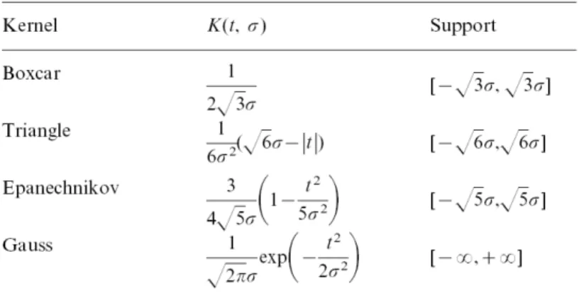
K(t) is required to be non-negative to avoid negative rates. Moreover, the ker-nel should be normalized such that each spike contributes with unit area to the rate function; this also guarantees that the integral of λ(t) is equal to the total number of spikes n recorded during the interval (0, T]. Finally, the first moment of K(t) is required to be zero to preserve the center of mass of the spike train.
Figure 3.3: Kernel functions
the estimated rate function. The kernel width is defined as
σ = s
Z ∞
−∞
t2K(t)dt (3.18)
which can be viewed as a smoothing parameter. Table 1 listed four kernel functions of different shapes, parameterized by their standard width.
The authors evaluated the rate estimators depending on shape and width of kernel functions, the integrated square error (ISE) is defined as
ISE =. Z T
0
(λ(t)−ρ(t))2dt (3.19)
density estimator, is most often used.
λ(t) = √ 1 2πσ2
n
X
i=1
exp
−(t−τi)
2
2σ2
(3.20)
When λ(t) varies slowly, Gaussian kernels do a good job of estimating the rate and filtering out the noise. Nevertheless, when the firing rate varies quickly, Gaussian fil-ters are not able to capture the variation without introducing artificial high-frequency fluctuations. In other words, to filter high-frequency noise, the Gaussian kernel den-sity estimator must remove the high-frequency firing rate.
In general, the most obvious advantage of kernel smoothing is its simplicity. Kernel smoothing methods are extremely fast and simple to implement. However, as the results depend critically on the choice of the smoothing parameter σ, the lack of a global choice of the bandwidth is typically considered a major shortcoming of kernel smoothing methods.
3.2.2
Adaptive Kernel Smoothing
There are two concerns about the standard fixed bandwidth kernel estimation. One is that it requires the investigator to choose the parameter σ arbitrarily, which produce significantly different estimates of firing rates. The other problem is that the bandwidth of the standard kernel estimator is constant throughout the time interval of the neuronal response. Richmond et al.(1990) tried to solve those two problems by varying the width of the estimation kernel throughout the trial, letting the data themselves determine how much to vary the width of the kernel. This process is called adaptive-kernel estimation, because the width of the kernel adapts to the local density of the data points (Richmond, 1990).
(i) Firstly, form a fixed bandwidth kernel estimate (called a pilot estimate) from the data, the bandwidth is σp;
(ii) Then, this pilot estimate of the density is used as a measure of the activity over small time periods throughout the entire response interval. The definition of ”small” here depends on the choice of the fixed kernel bandwidth, σp;
(iii) These local kernels are then used to produce a smoothed firing rate that changes more rapidly in regions of high firing, and less in regions of less firing.
The pilot estimate is used to define a set of local bandwidth factors, λi,
λi =
s
f(i)
µ (3.21)
where f(i) is the pilot estimate at the ith point, and µis the geometric mean of the pilot estimates,
µ= exp "
1
n
n−1
X
i=0
lnf(i) #
(3.22)
Finally, the adaptive kernel estimate is computed by convolving each point with a kernel density function having a width that is the product of the fixed bandwidth σp
and the factor for each point
m(k) = 1
n
n−1
X
0 K
t−τi|σ =
σp
λi
(3.23)
3.2.3
Kernel Bandwidth Optimization
Kernel smoother and a time histogram are classical tools for estimating an in-stantaneous firing rate.The optimization method was initially proposed for the joint
peristimulus time histogram(PSTH) of spike counts over multiple neurons (Shimazaki, 2007b). The method can select the bin width of the time histogram automatically based on the principal of minimizing the mean integrated squared error (MISE), de-fined as follows, without knowing the underlying rate.
M ISE =
Z T
0
E(λ(t)−λˆ(t))2dt, (3.24)
where λ(t) is the underlying rate and λˆ(t) is the estimation, and E refers to the expectation with respect to the spike generation process under a given time-dependent rate λ(t).
Similarly, we consider a kernel rate estimator as λˆ(t) and select the width of a kernel under the MISE criterion. Suppose independently and identically obtained m
spike trains which contain M spikes as a whole, then a superposition of the spike trains can be regarded as being drawn from an inhomogeneous Poisson point process, due to the general limit theorem of the sum of independent point process (Shimazaki, 2009). Let’s define ¯Yt= m1 PMi=1δ(t−τi0), whereτ
0
i is theith spike of the superimposed
spike sequence and δ(·) is still the Dirac delta function. The estimator λ(ˆt) can be constructed by a kernel function Kw(·) as λ(ˆt) =
R ¯
YsKw(t−s)ds, where w refers to
the bandwidth.
Following Equation 3.24, the integrand can be decomposed into three terms:
λ(t)2 −2λ(t)E( ˆλ(t)) +E( ˆλ(t)2). Since the first component does not depend on the
function of the bandwidth w,
Cm(w)
.
=M ISE−
Z T
0
λ(t)2dt =−2 Z T
0
λ(t)E( ˆλ(t))dt+ Z T
0
E( ˆλ(t)2)dt. (3.25)
From a general decomposition rule of a covariance of the two random variables, we obtain
Z T
0
λ(t)E( ˆλ(t))dt = Z T
0
E( ¯Ytλ(ˆt))dt−
Z T
0
E( ¯Yt−E( ¯Yt))( ˆλ(t)−E( ˆλ(t)))dt
=E
Z T
0
¯
Ytλ(ˆt)dt
− Kw(0)
n E
Z T
0
¯
Ytdt
.
(3.26)
To obtain the next equality, we used the assumption that the spike sequence is a Poisson process so that the spikes are independent to each other. Hence, the cost function is estimated as
ˆ
Cm(w) =
2Kw(0)
m
Z T
0
¯
Ytdt−2
Z T
0
¯
Ytλˆ(t)dt+
Z T
0
ˆ
λ(t)2dt
= 2Kw(0)
m2 M−
2 m2 M X i=1 M X j=1
Kw(τi0−τ
0
j) +
1 m2 M X i=1 M X j=1
ψw(τi0 −τ
0
j),
(3.27)
where ψw(t) is given by ψw(t)
.
=R0T Kw(s)Kw(s+t)ds.
The optimal bandwidth w∗minimizes the score function ˆCm(w).
3.2.4
Smoothing Splines
The penalty smoothing estimate the rate function by maximized the penalized likelihood function (Gu, 2008). We first consider a nonparametric regression problem
Yi =η(xi) +εi, i= 1,2, ..., n, where n is the total number of points of a spike train,
estimate η(·) via the penalized least square
1
n
n
X
i=1
(Yi−η(xi))2+κ
Z 1
0
(η00(x))2dx (3.28)
where the first term,Pn
i=1(Yi−η(xi)) 2
, measures the goodness-of-fit of the smoothing function η to the data, the second term, J(η) = R1
0 (η 00(x))2
dx, penalizes the rough-ness of η(x) and the smoothing parameter κ controls the trade-off between the two conflicting goals. The solution of (3.28) is known as natural cubic spline. Asκ→ ∞, the estimate ”shrinks” into the null space of the roughness penalty,{η :R01η00(x)dx}. When κ → 0, it converges to the minimum curvature interpolation, i.e. Yi = η(xi)
for i= 1,2, ...n.
For the point process data, log-likelihood is used as the goodness-of-fit measure, instead of the least square. As we known, when the error terms of the regression are assumed to be independent and identically distributed Normal random variables, ordinary least square (OLS) turns out to be equivalent to maximum likelihood esti-mation (ML).
Consider the so-called exponential family distributions with densities of the form
f(y|η, φ) = exp{(yη−b(η))/a(φ) +c(y, φ)}, (3.29)
where a > 0, b and c are known functions, η is the parameter of interest and φ is either known or considered as a nuisance parameter. Observing Yi f(y|η(xi), φ), one
may estimateη(x) via the general penalized likelihood,
−1
n
n
X
i=1
{Yiη(xi)−b(η(xi))}+κJ(η) (3.30)
A special case of the penalized likelihood method is for Poisson regression. For the density function f(y|η) = exp{yη−eη−logy!}, one may minimize the penalized likelihood
−1
n
n
X
i=1
Yiη(xi)−eη(xi) +κJ(η), (3.31)
where η(xi) = logλ(xi) is the log intensity and the λ(xi) > 0 but η(xi) is free of
Chapter 4
The Methods
Synchronized firing of related neurons is an interesting fact which motivates us to develop statistical analysis using the valuable information of concurrent spiking activities (or called peer activities). Our research focuses on applying and developing statistical approaches to analyze simultaneously recorded neural spike trains and in-fer functional connectivity between interactive neurons in brain. In this chapter, we introduce two models for spike train analysis: the first one is a point process likeli-hood method under the generalized linear model framework, and the second one is a proposed regression spline model for modeling both the spontaneous firing and also the influence of interactive nerve cells. Simulation results and real data applications will be presented in Chapter 5.
4.1
Continuous State-Space Model
assembly population than by using only external variables. There are three major steps in the method. Initially, all the peer spike trains are smoothed with a Gaussian filter in the time domain.
s(t)α= √ 1 2πσ2
nα
X
j=1
exp
−(t−τ
α j )2
2σ2
, (4.1)
where α is the index of peer cells, {τα
j } is the spike train of neuron α, and nα is the
number of spikes of peer α. σ is the smoothing bandwidth of the Gaussian kernel, termed peer prediction timescale by the author.
Then, under the generalized linear model, the predicted intensity function at time
t is given by
λ(t) =g(X
α
s(t)αwα), (4.2)
where wα is the prediction weight of peer α. The sign of the weight represents the positive or negative correlation between a certain member neuron and the target neuron. Here g(·) is the link function and has the following form
g(x) =
exp(x) x <0
x+ 1 otherwise
(4.3)
The advantage of this link function is that it will not lead to excessively high intensity when many positively correlated peer cells fire simultaneously compared with a simple exponential link function.
The final step is to estimate the weight by maximizing the penalized log-likelihood on the training set.
log(Lf) =
X
t
[−λ(t)∆ + ∆Ntlog(λ(t)∆)]−
1 4
X
α
The maximum is carried out by Newton’s method with an analytically calculated Hessian matrix.
A 10-fold cross-validation procedure is used to repeatedly divide the recorded data into a training set and a test set. For each training set, the mean firing rate is calcu-lated, f0 , as the number of spikes during the training period divided by the length
of the training period. The prediction quality on the test set, termed predictability, is defined as the difference, log(Lf)−log(Lf0), over the base of log(2). Then, the
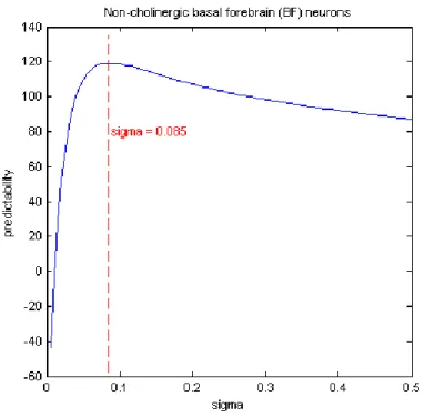
predictability of the entire data set is defined by a cross-validation procedure, where the data are divided into 10 segments, each segment is used in turn as test set, and the log likelihood ratios for each segment are summed and divided by the total time. As the spike train is smoothed by the Gaussian kernel, then the choice of the bandwidth,σ in Equation (4.1), is critical. In Harris (2003), the optimal bandwidth,
σ, is chosen by optimizing the predictability; therefore, it maximizes the log likelihood function, log(Lf), among all the values of σ.
4.2
Regression Spline Model
The spontaneous firing rate for one particular neuron depends on its own natural characteristics. Also, the firings of other neurons (also called peers) within the neural network have impacts on the target neuron. In this section, we propose a regression spline model for neural spike train data with interactive neural activities.
4.2.1
Model
Suppose there are M covariates and their firing times before time t are given by
x(t) = (x1(t), .., xM(t)). Let T be an nonnegative random variable ranging over a
and F(t|x) denote the conditional density and conditional distribution function, re-spectively, ofT givenx∈RM. Letλ(·|x(s)) denote the conditional intensity function
of T givenx(s) so that
λ(t|x(t))dt= P(T ∈(t, t+dt)|x(t)).
Letα(·|x(t)) denote the log conditional intensity function. To simplify the discussion, we assume that the conditional intensity function at time t depends on the value of the covariates only up to that time; that is, we assume that λ(t|x(s), s > 0) =
λ(t|x(s),0≤s≤t) and hence that α(t|x(s), s >0) = α(t|x(s),0≤s ≤t). In this paper, we model the log conditional intensity function via
α(t|x(t)) =µ(t) +β·Q(t|x(t)), t ≥0, (4.5)
where µ(t) is the baseline function which represents the spontaneous firing rate,
Q(·|·) = (Q1, ...QM) is the vector of M-dimensional polynomial functions which
de-scribe the effects of the covariates, and β = (β1, ..., βM) are the coefficients. This
model is flexible for an arbitrary number of interacting neurons. Brillinger (1988) gave a step function to approximate the peer effects on the target neuron. In our method, the components of Q(·|·) are all continuous functions whose explicit forms would be discussed in detail in Section 4.
Set x=x(t). The log-likelihood based on (T,x) is given by
l = logλ(T|x)− Z
λ(u|x)du=α(T|x)− Z
ind(T ≥u) expα(u|x)du
={µ(T) +β·Q(T|x)} − Z
ind(T ≥u) exp(µ(u) +β·Q(u|x))du.
The expected log-likelihood is given by
E
logλ(T|x)− Z
ind(T ≥u)λ(u|x)du
=
Z
[logλ(t|x)f(t|x)−(1−F(t|x))λ(t|x)]dt.
Letτ1, ...τnbe independent random variables having distribution functionsF(·|xi),
and let xi ∈RM denote the vector of covariates for the ith individual, 1≤i≤n. Let
G denote a linear space of polynomial spline functions on T. Let function h(t|xi) =
g(t) +β·Q(t|xi), where g ∈G. The expected log-likelihood function Λ(·) is defined
by
Λ(h) =X
i
Z
[h(t|xi)f(t|xi)−(1−F(t|xi)) exph(t|xi)]dt.
Observe that Λ(·) is maximized at α = log(f /1− F) = µ+β ·Q. µ(t) may or may not be in G, but we can define the best approximation to µ, µ∗ ∈ G, so that
α∗ =µ∗+β·Q maximizes Λ(·) over G.
The best approximation will be chosen from the linear spaceG. Say for 1≤p <∞ the baseline function in Model 4.5 is spanned by the B-spline functions: B1, ..., Bp,
and
α(t|x) =
p
X
i=1
θiBi(t) +β·Q(x), t≥0, (4.6)
where θ= (θ1, ..., θp) are the coefficients for pbasis functions.
is necessary that the dimension p of the approximation space G tend to infinity. To control the error of estimation, we need this dimension to increase more slowly than
n1/2.
The model aggregates the influences from peers using polynomial functions, and each covariate extends the model in terms of adding a polynomial term. The aggre-gating methodology offers high flexibility for real situations. In this paper, we will see the applications for applying different order functions for single or multiple covari-ates, and also we will discuss how to explain the applications in realistic cases later. For illustration purposes, we now use a special case with the polynomial function of order 1 to describe our proposed methodology. Equation 4.7 is a simplified version of 4.6 with only one covariate. The general case with multiple covariates is just a straightforward extension.
α(t|x(t)) =
p
X
i=1
θiBi(t) +β1Q1(t|x1(t)), t≥0. (4.7)
4.2.2
Maximum Likelihood Estimation
Given the vector of covariates x(t) and the baseline function spanned by a set of basis functions, B= (B1, ..., Bp), we can estimate the coefficients in Equation 4.7 by
maximum likelihood. The partial log-likelihood for a neuron can be written as
φ(t|x(t)) = logλ(t|x(t))− Z t
0
We take the partial derivatives ofφ(·) to examine its concavity and maximize the log likelihood. Set
Djθ = ∂Λ(t|x)
∂θj
= Z t
0
Bj(s) exp (θ·B(s) +β·Q(s|x))ds forj = 1, ..., p,
Dkβ = ∂Λ(t|x)
∂βk
= Z t
0
Qk(s|xk(s)) exp (θ·B(s) +β·Q(s|x))ds for k = 1, ..., M,
(4.9)
and
Ej,lθ = ∂
2Λ(t|x(t)) ∂θj∂θl
= Z t
0
Bj(s)Bl(s) exp (θ·B(s) +β·Q(s|x))ds
for j, l = 1, ..., p, Ej,kθ,β = ∂
2Λ(t|x(t)) ∂θj∂βk
= Z t
0
Bj(s)Qk(s|xk(s)) exp (θ·B(s) +β·Q(s|x))ds
for j = 1, ..., p and k= 1, ..., M, Ek,qβ = ∂
2Λ(t|x(t)) ∂βkβq
= Z t
0
Qk(s|xk(s))Qq(s|xk(s)) exp (θ·B(s) +β·Q(s|x))ds
for k, q = 1, ..., M.
(4.10)
Then
∂φ ∂θj
=Bj(t)−Dθj,
∂φ ∂βk
=Qk(t|xk(t))−Dkβ,
∂2φ ∂θj∂θl
=−Ej,lθ , ∂ 2φ
∂θj∂βk
=−Ej,kθ,β, ∂ 2φ
∂βkβq
=−Ek,qβ .
(4.11)
It follows from Equation 4.11 thatφ(t|x(t)) is a concave function. Hence there exists a unique maximum likelihood estimate ˆh= ˆθ·B ∈G[see Kooperberg et al. (1995b)] and ˆβ so that [ˆθ,βˆ] = maxl(θ,β).
generated by individual neurons, and the typical form of a neural spike train is a temporal point process that shows precisely the times of firing. The interval between two consecutive firings as shown in Figure 5.13 are referred to as interspike interval (ISI), and here we denote the interspike intervals for a spike train with N spikes as {uk}Nk=1.
The log-likelihood function is a sum for all N consecutive ISIs {uk}Nk=1 given by
l(θ, β1) =
N
X
k=1
α(uk|x(uk))− N
X
k=1
Z uk
0
λ(s|x(s))ds (4.12)
The maximum likelihood estimate bθ and βb will be obtained by maximizing the log-likelihood, l(θ,β).
Under certain conditions, Kooperberg, Stone and Truong (1993) obtained the L2
rate of convergence in estimating the log intensity function.
4.2.3
Adaptive Model Selection
A useful feature in this model for neural spike train analysis is that the spaceGof approximation is chosen adaptively. This can be really useful in capturing respective features of firing rate for various neurons in a large network. The methodology is similar in spirit to MARS (multivariate adaptive regression splines), and the choice of the space G and its dimension pare resolved adaptively.
The selection of the dimension and the basis functions of G employs stepwise addition and stepwise deletion of basis functions. Initially, we use minimal allowable space to model α(t|x(t)), so that the one dimensional model is fit. Then we proceed with stepwise addition, successively replacing a (p−1)-dimensional spaceG0 by ap
-dimensional space Gthat contains G0 as a subspace. At each step a candidate basis
heuristic search, which maximizes the Rao statistics.
The addition would be stopped when one of the following conditions is satisfied; see Kooperberg et al. (1995) for detail.
1. The number P of basis functions equals Pmax, where the default value for Pmax
is min(4n1/5,n/4,30).
2. The search algorithm yields no possible new basis function.
3. ˆlP − ˆlp < 12(P − p) −0.5 for some p with 3 ≤ p ≤ P −3, where ˆlp is the
log-likelihood for the model withp basis functions.
Upon stopping the stepwise addition stage, we proceed to stepwise deletion by successively replacing the p-dimensional allowable space G by a (p−1)-dimensional allowable subspace G0 until we arrive at the minimal allowable space. For each step,
the basis function that would be removed in going from G to G0 has the smallest
Wald statistic in space G. The Rao statistics during the stepwise addition and Wald statistics during the stepwise deletion give an approximation of the change in the log-likelihood due to adding or deleting a basis function that does not require finding the new maximum likelihood estimation of parameters.
During the combination of stepwise addition and deletion, we get a sequence of models. Letpν denote the number of parameters and ˆlν be the log-likelihood of theνth
Chapter 5
Numerical Studies
This chapter presents the simulation results and real data applications according to the methods introduced in Chapter 4. Section 5.1 and 5.2 follow the models in Section 4.1 and Section 4.2 respectively.
5.1
Continuous State-Space Model
5.1.1
Simulation
First, we consider the simplest situation, when there is only one peer with the target spike train. To test the prediction methods when the true underlying firing rate is known asλ1(t), we simulated two inhomogeneous Poisson spike trains positively
correlated with weight 3, the target spike train with rateλ1(t) ,and its peer with rate λ2(t), so that λ1(t) = 3∗λ2(t) + 1 for all time t from 0 to 50 seconds. Both the
training and testing sets are generated in the same way.
Figure 5.2: The underlying firing rate function.
To select the optimal σ, the procedure was repeated 100 times given each σ fixed. We got 100 estimated weights, and the kernel density function of those 100 w’s is plotted in Figure 5.3. For σ from 0.1 to 2, σ= 5.3 has the kernel density with mean 3, which is the true weight of the peer. So, from the estimated weight, the optimal timescale is 5.3. Thisσ= 5.3 is also the optimal choice by the maximal predictability criteria.
For Figure 5.4, the x axis is σ from 0.1 to 2, and the y axis is the counts of those optimal σ’s where the predictabilities achieve the maxima. The kernel density function is skewed, and the median is 5.35. So, from both the estimated weights and predictabilities, the optimal peer prediction timescale is 5.3, and it was used to predict the target spike train in the testing data set.
Figure 5.3: The kernel density follows approximately normal distribution. The density of σ = 5.3 has mean 3 which is the true weight of the peer.
Figure 5.5: The blue solid curve in the middle is the underlying firing rate function, the red solid curve is the mean curve of 100 predicted intensity functions, and the black solid curve is the mean curve of the intensity functions of the 100 spike trains in the testing set. Red and black dashed lines are the 95% boundaries for the predictions and smoothing functions respectively.
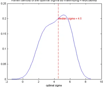
When we have multiple peers, we cannot select the optimal σ from estimated weights, but the maximal predictability criteria still works well. Keeping the under-lying rate function of the target spike train unchanged, two unequally weighted peers are generated with weight 1 and 2 respectively. Figure 5.6 shows the kernel density of the optimal σ’s in terms of maximizing the predictability of those two peers, and we can see the median is σ= 4.5.
Finally, we can still have unbiased prediction by setting σ = 4.5 in the two peer case. The unbiasedness is shown in Figure 5.7.
5.1.2
Real Data Analysis
Figure 5.6: Kernel density function of 100 optimal σ’s in terms of maximizing the predictability.
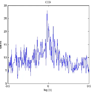
Another spike train from neuron 5 that is positively related to the target spike train was selected as the first peer to predict the firing rate of neuron 1. Figure 5.9 is the cross-correlogram (CCG) which peaks at lags close to 0. An intuitive interpretation of the CCG is that the target neuron is more likely to fire immediately before or after the peer. We can expect an positive weight estimated between this target neuron and its peer due to the synchronous firing.
Figure 5.9: Cross-correlogram of neuron 1 (the target neuron) and neuron 5 shows a peak for lags that are less than 0.1 second.
or one of them (neuron 15) has no significant correlation with the target neuron.
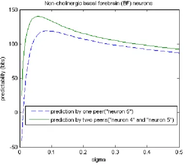
Figure 5.10: Both neuron 4 and neuron 5 are positively correlated to the target neuron. Predictabilities were estimated by one peer (neuron 4) or two peers (neuron 4 and neuron 5). Prediction by those two peers save more information bits overall.
Neuron 4 has an excitatory impact on the the target neuron as well. When we estimate the rate function based on the two peers (neuron 4 and neuron 5), we can see in Figure 5.10 that the green curve overall is above the blue one which is the predictability from one peer (neuron 5) only.
What if we involve another spike train that has no strong evidence to the syn-chronization with the target spike train? We can see in Figure 5.11(b) that involving neuron 15, which has no correlation with the target neuron, does not improve the predictability.
Figure 5.12: Predictability versus peer prediction timescale for peer neuron 5. The optimal bandwidth for prediction is 0.085 seconds.
5.2
Regression Spline Model
two neurons have dramatically different rates of firing or the resting period of one neuron is significantly longer than some others. For these cases, we need to allow more flexibility of the covariate terms; say for a certain target, more spikes from each peer will be considered in the model. Section 5.2.7 gives a real application as we just described; that section also embeds the details of the model selection using AIC to select the appropriate number of firings for each peer.
Simulation studies are conducted to validate the method in Sections 5.2.2 and 5.2.3 and to compare the results with Brillinger’s approach for the spline estimation in Section 5.2.4. Section 5.2.1 starts with the generation of a neural spike train in which we introduce a general algorithm for a given conditional intensity function. We obtain correlated spike trains linked through the covariates terms in model 4.6. We then estimate the parameters in two stages. In 5.2.2, the knot numbers and locations of the spline are fixed, and the optimization is a simple MLE problem for the fixed knot case. If the knot locations are also to be optimized, we apply the adaptive model selection scheme in 5.2.3. We observe that both the spline fit with either fixed or adaptive knots can give almost unbiased estimates, and we observe that the kernel density of the estimations is approximately normal.
5.2.1
Simulation Study I: A General Algorithm of Neural
Spike Train Generation
(called bins), ∆. The bins need to be sufficiently small compared to the actual ISI. For example, if the actual ISI is expected to be around 1 second, then the bin size should not be larger than 1 millisecond.
2. For any given sets of spline knots (t1, ..., tp), coefficients (θ1, ..., θp), peer spike
times, and the coefficientβ1, we can calculate the log-intensity for each bin, one
at a time. Beginning at time 0, the log-intensity for the first bin is α(∆|v1) =
Pp
j=1θjBj(∆) +β1[K −(∆−v1)]1∆≥v1. The first spike of the peer does not
impact the log-intensity function if v1 >∆.
3. After taking the logarithm of the log-intensity function, the probability of one event occurring within the interval ∆ equals the product of the intensity function and ∆ (see Equation 2.10).
4. A random number is drawn following a Bernoulli distribution and the proba-bility is what we calculated by step 3: 0 for no occurrence and 1 for one spike occurrence in the small interval.
5. If the outcome of the Bernoulli trial fails, we move onto the next bin and the time in step 2 is accumulated, from ∆ to 2∆, or from 2∆ to 3∆, and so on, until a time at which the Bernoulli trial succeeds.
6. If the outcome of the Bernoulli trial succeeds, the time is reset back to 0, and we move onto the next available spike of peer as the covariate and repeat step 2 to 5.
However, it is still not trivial to obtain the simulated sequences with correlation as desired. Let’s see an example. The design of the example requires that the inter-spike interval for the target neuron contains exactly one peer firing. In other word, the target neuron is less likely to fire until the peer fires, and such impact is strong enough to trigger one target firing almost sure. The spontaneous firing rate, therefore, is set to be close to 0, and the increment of the intensity due to peer activity will raise rapidly as the lag time increases. To control the consecutive firings and make the repetitions behave similarly and stably, the ISI of the peer can be set as a constant without loss of generality.
Similar design can be easily extend to more sophisticated cases, like multiple peer effects or negative peer effects.
5.2.2
Simulation Study II: Fixed-Knot Splines
We follow the principle ideas in an “integrate-and-fire” model. Stimulus from peers in the form of current inputs are accumulative until the next firing of target cell. After that triggering, the stimulus before would have no impact on any coming events, such as resetting the clock and counting from zero. In the meantime, the voltage of the membrane naturally decays along the time so that the impact of peer firing diminishes gradually, referred to as “leaky integrate-and-fire”. Based on those neurobiological supports, we proposed a model of interspike interval (ISI) data which follows Equation 4.7 while Qis a decreasing function of time.
For two interacting neural spike trains, the target spike train has N spikes or N
ISIs, {uk}Nk=1. Then each spike of the peer belongs to an individual ISI of the target
spike train and only affects the target within that interval. So, for any uk, we denote
When more than one spike of a peer occur within an ISI of target spike train, we consider only the last one as the covariate.
Figure 5.13: Target and peer spike trains are recorded simultaneously. Between two consecutive spikes of the target, the distance is our observation and uk is for the
interval ending at the kth spike. The peer may fire within the interval, and then we record the distance from the beginning of uk to the peer firing time as our covariate
vk.
The conditional log-intensity function for the kth observation is
α(t|vk) = p
X
i=1
θiBi(t) +β1[K −(t−vk)]1t≥vk, t≥0, (5.1)
where 1t≥vk is an indicator function andK is a constant that is deterministic for each
target spike train. In the model, the target spike train keeps its spontaneous firing rate before it is stimulated by the peer firing. Therefore the covariate term is zero untilt ≥vk.
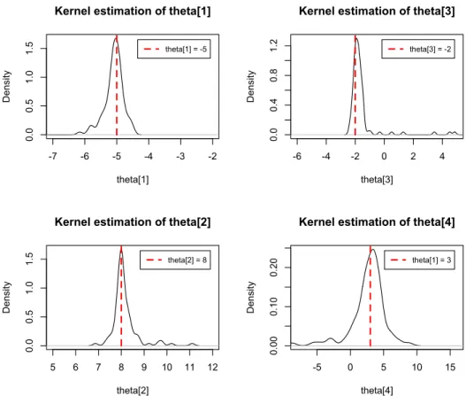
Following the recipe above, we simulated 100 spike trains, each of which has 650 spike times given a deterministic peer spike train. In Figure 5.14 and Figure 5.15, the estimators of θ1 to θ4 correspond to knot locations {0.2,0.4,0.6,0.8} and the
estimator of β1 are shown respectively after 100 simulations.
-7 -6 -5 -4 -3 -2
0.0
0.5
1.0
1.5
theta[1]
D
en
si
ty
Kernel estimation of theta[1]
theta[1] = -5
5 6 7 8 9 10 11 12
0.0
0.5
1.0
1.5
theta[2]
D
en
si
ty
Kernel estimation of theta[2]
theta[2] = 8
-6 -4 -2 0 2 4
0.0
0.4
0.8
1.2
theta[3]
D
en
si
ty
Kernel estimation of theta[3]
theta[3] = -2
-5 0 5 10 15
0.00
0.10
0.20
theta[4]
D
en
si
ty
Kernel estimation of theta[4]
theta[1] = 3