A generalized Poisson and Poisson-Boltzmann solver for electrostatic environments
G. Fisicaro, L. Genovese, O. Andreussi, N. Marzari, and S. Goedecker
Citation: The Journal of Chemical Physics 144, 014103 (2016); doi: 10.1063/1.4939125 View online: http://dx.doi.org/10.1063/1.4939125
View Table of Contents: http://scitation.aip.org/content/aip/journal/jcp/144/1?ver=pdfcov Published by the AIP Publishing
Articles you may be interested in
Ionic screening of charged impurities in electrolytically gated graphene: A partially linearized Poisson-Boltzmann model
J. Chem. Phys. 143, 134118 (2015); 10.1063/1.4932179
An ionic concentration and size dependent dielectric permittivity Poisson-Boltzmann model for biomolecular solvation studies
J. Chem. Phys. 141, 024115 (2014); 10.1063/1.4887342
Electrostatic forces in the Poisson-Boltzmann systems J. Chem. Phys. 139, 094106 (2013); 10.1063/1.4819471
Adapting Poisson-Boltzmann to the self-consistent mean field theory: Application to protein side-chain modeling
J. Chem. Phys. 135, 055104 (2011); 10.1063/1.3621831
A modified Poisson–Boltzmann analysis of the capacitance behavior of the electric double layer at low temperatures
J. Chem. Phys. 123, 034704 (2005); 10.1063/1.1992427
A generalized Poisson and Poisson-Boltzmann solver
for electrostatic environments
G. Fisicaro,1,a)L. Genovese,2O. Andreussi,3,4N. Marzari,4and S. Goedecker1
1Department of Physics, University of Basel, Klingelbergstrasse 82, 4056 Basel, Switzerland 2University of Grenoble Alpes, CEA, INAC-SP2M, L_Sim, F-38000 Grenoble, France 3Institute of Computational Science, Università della Svizzera Italiana, Via Giuseppe Buffi13,
CH-6904 Lugano, Switzerland
4Theory and Simulations of Materials (THEOS) and National Centre for Computational Design
and Discovery of Novel Materials (MARVEL), École Polytechnique Fédérale de Lausanne, Station 12, CH-1015 Lausanne, Switzerland
(Received 2 September 2015; accepted 6 December 2015; published online 6 January 2016)
The computational study of chemical reactions in complex, wet environments is critical for appli-cations in many fields. It is often essential to study chemical reactions in the presence of applied electrochemical potentials, taking into account the non-trivial electrostatic screening coming from the solvent and the electrolytes. As a consequence, the electrostatic potential has to be found by solving the generalized Poisson and the Poisson-Boltzmann equations for neutral and ionic solutions, respectively. In the present work, solvers for both problems have been developed. A preconditioned conjugate gradient method has been implemented for the solution of the generalized Poisson equation and the linear regime of the Poisson-Boltzmann, allowing to solve iteratively the minimization problem with some ten iterations of the ordinary Poisson equation solver. In addition, a self-consistent procedure enables us to solve the non-linear Poisson-Boltzmann problem. Both solvers exhibit very high accuracy and parallel efficiency and allow for the treatment of periodic, free, and slab boundary conditions. The solver has been integrated into the BigDFT and Quantum-ESPRESSO electronic-structure packages and will be released as an independent program, suitable for integration in other codes. C 2016 AIP Publishing LLC.[http://dx.doi.org/10.1063/1.4939125]
I. INTRODUCTION
Many important chemical processes take place in solution both in the context of basic and industrial research. The computational study of such chemical reactions in wet environments is therefore of cross-disciplinary interest to physics, chemistry, materials science, chemical engineering, and biology.1 Computational studies can complement these investigations by giving insight into new processes and materials as well as reducing development times and production costs. Solar-energy harvesting in a dye-sensitized cell or electro-catalytic water splitting are two simple examples of relevance for applications in the energy and environment context.
Molecular properties in the presence of a solution are often very different compared to purein vacuum2conditions making vacuum-like ab initio calculations an inappropriate approach for such problems. An inclusion of the solute-solvent interaction inab initiosimulations is thus mandatory. On the atomistic scale, an explicit inclusion of all solvent molecules in the simulation should be in principle the natural way to account for solvent effects. Due to the very large number of water and possibly other molecules required, this approach enormously increases the computational cost and limits at the same time the size of the system contained in the explicit dielectric medium.3 The study of the
solute-a)[email protected]
solvent interaction at length scales larger than the molecular sizes would become virtually impossible. Investigations like structure predictions4 or reaction path determination5would become unaffordable in such a purely atomistic approach. Moreover, fully atomistic simulations of solvation effects would need to deal with the extensive sampling, required to characterize liquid configurations, and with the well-known limitations that current state-of-the-art ab initio methods present in describing liquid water, in particular regarding its structural and dielectric properties.
An implicit inclusion of the solute-solvent interactions can solve these issues. Starting from the earliest work of Onsager,6 the quantum chemistry community investigated implicit solvation models7–9 extensively. In these models, the solvent is introduced as a continuous homogeneous and isotropic medium fully described by a dielectric function. Among them, the polarizable continuum model (PCM) developed by Tomasi and co-workers7,8 is one of the most popular models. In this approach, a dielectric cavity surrounding the atomistic system is introduced where the permittivity takes on the value of one in regions occupied by atoms and some different value characteristics for the dielectric solvent medium considered outside.
Density functional theory (DFT) is a widely used method to investigate material properties at the atomistic scale. In suchab initiocalculations, the electronic-structure problem is solved by minimizing the total energy of the system which is a functional of the electronic density
0021-9606/2016/144(1)/014103/12/$30.00 144, 014103-1 © 2016 AIP Publishing LLC
E[ρ]=T[ρ]+
v(r)ρ(r)dr+1 2
ρ(r)φ[ρ]dr+Exc[ρ],
(1)
where the four terms on the right side of Eq. (1) are, respectively, the standard kinetic energy, the interaction energy with an external potential, the electrostatic and the exchange-correlation energies. For gas-phase molecular simulations, the potential φ(r) generated by a given charge density ρ(r) is given by the solution of the standard Poisson (SPe) equation
∇2φ(r)=−4π ρ(r). (2)
An implicit inclusion of the solvent at such DFT level can be obtained by introducing a continuum dielectric cavity by means of a dielectric distributionϵ(r). Then, the potential is given by the solution of the generalized Poisson equation (GPe)
∇ ·ϵ(r)∇φ(r)=−4π ρ(r). (3)
If the system is surrounded by an ionic solution, an extra-term has to be added on the right side of Eq. (3). It accounts for the ionic distribution in the liquid and depends on the local electrostatic potentialφ(r). The resulting non-linear differential equation would therefore become
∇ ·ϵ(r)∇φ(r)=−4π ρ(r)+ρions[φ](r),
(4)
whereρions(r)is the local concentration of ions in the dielectric solvent, written as a sum of concentration contributionsci of
ions of type i∈{1,2, . . . ,m}and valence Zi, which in turn
areφ-dependent functionals,
ρions
[φ](r)=γ[ϵ](r)eNA m
i=1
Zici[φ](r). (5)
Here,eis the elementary charge,NAthe Avogadro’s number,
and γ[ϵ](r)a proper function which guarantees that mobile ion concentrations tend to zero inside the dielectric cavity mapped by ϵ(r). The most common expression for the ci[φ]
functional gives rise to the well-known Poisson-Boltzmann equation (PBe).
Whereas several approaches and solvers exist for the SPe,10–14 efficient and accurate solvers are still missing for the GPe and PBe cases. Some of these solvers handlesparse matrices obtained by low-order finite difference discretization of Eq. (3), many of them keeping constant the permittivity in both inner and external regions of the dielectric cavity and then solving a standard Poisson problem. Furthermore, simpler and linearized forms of the Poisson-Boltzmann equation are usually considered, neglecting steric effects and overestimating ionic concentrations close to highly charged surfaces and for multivalent ions.
Fast and accurate GPe and PBe solvers which accurately work for a continuously varying dielectric function could therefore play a key role in the extension of vacuum-based atomistic packages and allowing for quantum simulations in the presence of water, dissolved species, electrolytes, and non-aqueous solvents.
In the present paper, we present a minimization technique which solves the generalized Poisson problem and the linear regime of the Poisson-Boltzmann in some ten iterations of a
SPe solver. In combination with a self-consistent procedure, it enables us to solve the non-linear Poisson-Boltzmann problem in a formulation which includes ionic steric effects. The implemented algorithms take advantage of the chosen preconditioner for the minimization procedure. The accuracy of both GPe and PBe solvers has been tested for cases where an analytic solution is available. Two different methods have been implemented to describe the solvent surrounding the atomistic system. We prove the effectiveness of our method in practical DFT calculations of electrostatic solvation energies of various test systems.
II. GENERALIZED POISSON EQUATION
As discussed above, the dielectric medium is described by means of a position-dependent dielectric distributionϵ(r). In order to solve numerically Eq. (3), the potential φ(r), the charge density ρ(r), and the dielectric function ϵ(r)are generally discretized on a finite grid. In principle also, the generalized Poisson operator
A=∇ ·ϵ(r)∇ (6)
should be discretized on the same mesh. It will be shown that depending on the adopted strategy to solve numerically Eq. (3), the discretization of the differential operatorA can be avoided in exchange of an iterative procedure based on a SPe solver.
An alternative would be to solve the GPe iteratively as suggested in Ref. 15. In this approach, the polarization field introduced by the spatially varying dielectric function is added as a source term to the charge density of the ordinary Poisson equation, and the Poisson equation is solved repeatedly until self-consistency between the potential and the polarization charge density induced by it is reached. Our approach completes and simplifies this treatment, reducing considerably the number of SPe iterations, thereby presenting a robust and powerful iterative solver.
Considering that reliable convergence can be an issue in mixing schemes, an alternative approach based on a minimization procedure is desireable. Such an approach can be based on an action integral whose Euler Lagrange equation is the GPe [Eq.(3)],
I=
1
2∇φ(r)ϵ(r)∇φ(r)−4π ρ(r)φ(r)
dr. (7)
Any numerical minimization scheme can then be applied to solve the electrostatic problem.
In Sec. II B, our strategy to solve Eq. (3), based on a preconditioned conjugate gradient (PCG) algorithm, will be presented. The chosen preconditioner exactly represents the operator in the limit of a slowly varying dielectric constant and is based on the standard Poisson solver of BigDFT.
The possibility of solving the generalized Poisson equation under various boundary conditions (BCs) will be very important. In our approach, the boundary conditions enter in a straightforward way by means of the preconditioner, i.e., through the solution of the SPe.
ALGORITHM 1. Self-consistent (SC) iterative procedure.
1: setρiter 0
2:fork=0,1, . . .do
3: ρt o t k =ρ/ϵ+ρ
iter k
4: solve∇2φk=−4πρt o tk
5: ρiter k+1=
1
4π∇lnϵ· ∇φk
6: ρiterk+1=ηρkiter+1+(1−η)ρiter k
7: rk+1=ρiterk+1−ρiterk 8:end for
A. Self-consistent iterative procedure
A strategy to solve the GPe for a given charge densityρ(r)
is by means of a self-consistent (SC) iterative procedure.15 Applying simple algebraic manipulations, Eq. (3) can be rewritten as
∇2φ(r)=−4π
ρ
(r)
ϵ(r) +ρ
iter
(r)
=−4πρ(r)+ρpol(r)
, (8)
where ρpol(r) is the polarization charge density. In this approach, an extra-term ρiter(r),
ρiter
(r)= 1
4π∇lnϵ(r)· ∇φ(r) (9) induced by the spatially varying dielectric function ϵ(r) is added as a source to the charge density of the ordinary Poisson equation. Hence, the GPe can be solved by a self-consistent loop on the potential φ(r), obtained by a SPe solver onto the second member of Eq. (8). The residualrk, quantifying
the convergence, is the difference between the extra terms of Eq.(9)between subsequent iterations. Algorithm1describes the procedure. This approach requires a finite difference filter to be applied at step 5. In order to stabilize the iterative method, a linear mixing of the extra-term ρiter(r) at steps kth and(k+1)th has been introduced tuned by means of the mixing parameterη.
The polarization charge induced in the dielectric medium can be easily related to the extra-term of Eq.(9),
ρpol
(r)=ρiter
(r)+1−ϵϵ(r)
(r) ρ(r). (10)
This charge represents the response of the surrounding implicit dielectric. It lies in the transition region between the inner and outside parts of the cavity and stabilizes the solute density enveloped by the solvent.
B. Preconditioned conjugate gradient
Although a reasonably small number of iterations can be obtained in a self-consistent scheme, minimization techniques can produce more efficient methods to handle Eq. (3) if sophisticated schemes are utilized. In addition, the formulation as a minimization problem would allow to better control the convergence behavior.
Solving this equation with a preconditioned steepest descent (PSD) method is essentially identical to the self-consistency approach of Sec. II A, once a standard Poisson solver is taken as preconditioner. In particular, a good preconditioner for a PSD minimization, whose inverse applied
ALGORITHM 2. Preconditioned conjugate gradient (PCG).
1:r0=−4πρ− Aφ0,p−1=0 2:fork=0,1, . . .do
3: vk=P−1rk
4: pk=vk+βkpk−1(whereβk= ( vk,rk) (vk−1,rk−1),k,0)
5: αk= ( vk,rk) (pk,A pk)
6: φk+1=φk+αkpk
7: rk+1=rk−αkApk
8:end for
to a residual vectorrkprovides the preconditioned residualvk,
is as follows:
PSDvk(r)=ϵ(r)∇2vk(r)=−4πrk(r). (11)
Being the Laplacian ofvk(r)related to the residual vector
rk by means of Eq. (11), the generalized Poisson operator
becomes
Avk(r)=∇ ·ϵ(r)∇vk(r)=∇ϵ(r)· ∇vk(r)−4πrk(r). (12)
Such a PSD approach can be described by Algorithm2 with βk=0. Fixingαk=η, it corresponds to the previously
described self-consistent approach.
In a PSD scheme, the number of iterations l needed for convergence is proportional to the condition number κ (i.e., the ratio between the largest and the smallest eigenvalue of the product operatorP−1A). Minimization methods with
a faster convergence rate than the preconditioned steepest descent algorithm can significantly improve the convergence speed.
We use a preconditioned conjugate gradient scheme, where l∝√κ. In such minimization procedure, a good preconditioner can lowerκand, therefore, the overall number of iterations. Algorithm 2 describes the implemented PCG procedure to compute the electrostatic potentialφ(r)starting from a given charge densityρ(r). The minimization procedure starts from an initial gradientr0computed on an input guess
φ0.P is the preconditioner whose inverse has to be applied
to the residual vectorrkreturning the preconditioned residual
vk, and, finally,φkis the solution of Eq.(3). The convergence
criterion is imposed on the Euclidean norm of the residual vectorrk.
Both performances and accuracy in a PCG scheme criti-cally depend on the preconditioner chosen. We implemented a preconditioner based on the solution of the standard Poisson equation (namely, on a standard Poisson solver). Once a residual vectorrk is given at the step 3 of Algorithm 2, we
define a preconditioned residual from the following equation:
PCGvk(r)=
ϵ(r)∇2[vk(r)
ϵ(r)]=−4πrk(r). (13)
This equation has to be solved with respect tovk(r)oncerk(r)
is given.
In addition to speeding up the PCG procedure, the preconditioner defined by Eq. (13) retains a further feature which guarantees accuracy and fast performance for the whole electrostatic solver. In step 7 of Algorithm2, we have to apply the generalized Poisson operator A to the preconditioned residue pk, which means, thanks to step 4, applying it to vk.
Using a change of variable vk′(r)=ϵ
(r)vk(r), the GPe
becomes
∇ ·ϵ(r)∇vk(r)=
ϵ
(r)∇2vk′(r)−vk′(r)∇2ϵ(r). (14)
Now simple algebraic manipulations and Eq. (13)allow to rewrite the generalized Poisson operatorAas
Avk(r)=∇ ·ϵ(r)∇vk(r) (15) =−vk(r)q(r)−4πrk(r), (16)
where q(r)=ϵ(r)∇2ϵ
(r) is calculated once at the beginning of the PCG procedure and kept fixed for the whole minimization loop. Therefore, thanks to the chosen preconditioner, the action of the operatorAcan be simplified to a simple multiplication between the potential vk(r) and
the vector q(r) related to the spatially varying dielectric functionϵ(r). This feature, which provides the exact operator output, makes our PCG procedure robust and fast, avoiding any finite difference differentiation. Furthermore, reducing the PCG algorithm to simple vector operations makes its parallelization straightforward, delegating it to the chosen SPe solver. A similar discussion holds for the boundary conditions, which enter in a natural way by means of the preconditioner, i.e., through the solution of the ordinary Poisson equation, both in the SC and PCG algorithms.
C. Numerical results
Both the self-consistent iterative procedure (Algorithm1) and the preconditioned conjugate gradient minimization scheme (Algorithm 2) have been implemented and tested.
As SPe solver (step 4 of Algorithm 1 and step 3 of
Algorithm 2), we used the Interpolating Scaling Function (ISF) Poisson solver, allowing to obtain highly accurate electrostatic potentials for free, wire, surface, and periodic boundary conditions at the cost of O(Nlog(N)) operations, whereNis the number of discretization points (see Ref.14).
To test both solvers, analytic three dimensional functions have been used. An orthorhombic grid of uniform mesh spacinghgridand(nx,ny,nz)points in each directions has been
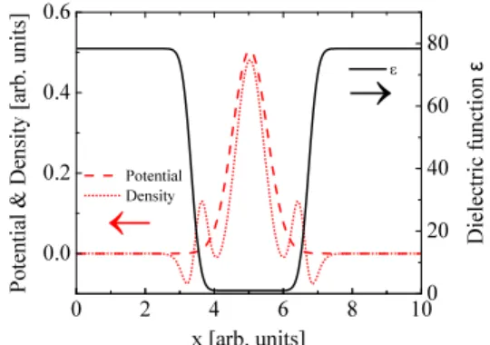
used. Fig. 1 shows plots of these benchmark fields along a particular direction passing through the box center and parallel to the y axis. All functions depend on the radial distance r from the center of the simulation domain.
A normalized Gaussian function has been chosen for the electrostatic potential φ(r) (red dashed line in Fig. 1) and the charge density ρ(r) has been derived from the chosen potential and dielectric functions, applying the generalized Poisson differential operator of Eq. (6) (red dotted line). In order to reproduce the dielectric environment typically tackled in electrostatic problems where a solute system is embedded in a solvent (i.e., a cavity where the majority of the atomic charge density is confined), the error function 1+(ϵ0−1)h(d0,∆;r)
has been chosen to represent the spatially varying dielectric constantϵ(r)(solid black line in Fig.1), where
h(d0,∆;r)=
1 2
1+erf (
r−d0
∆ )
. (17)
Here, ∆is a parameter which controls the transition region (≈4∆wide) between the inner and external parts of the cavity
FIG. 1. Analytical three dimensional functions used as benchmark fields for both SC and PCG solvers along a particular direction passing through the box center and parallel to the y axis. Red dashed line: potentialφ(r); red dotted line: charge densityρ(r); black solid line: dielectric functionϵ(r).
of radiusd0, andϵ0is the dielectric constant of the surrounding
medium. These benchmark functions have been used for both free, surface and periodic boundary conditions.
To implement the nabla differential operator needed for Algorithm1, central, forward and backward finite difference filters of order 16 have been used, which match the accuracy of the underlying SPe solver. We remark that the use of these finite difference filters is not needed for Algorithm2as soon as the vectorq(r)of Eq.(16)is pre-calculated.
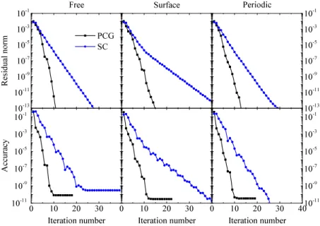
Fig. 2 shows solver performances. Top graphs report the residual norm as function of the iteration number. The residual norm is defined has the Euclidean norm of the residual vectorrk. Graphs in lower panel present the output
accuracy as a function of the iteration number. The accuracy in the whole paper is defined as the maximum value of the difference between the final numerical solution and the analytical potential. In this test case, a cubic box of length 10 a.u. has been chosen withnx=ny=nz=300. The Gaussian
variance for the potentialφ(r)wasσ=0.5, and the parameters of ϵ(r)were d0=1.7, ∆=0.3, and ϵ0=78.36 (all in a.u.).
The mixing parameter in step 6 of Algorithm1has been fixed to beη =0.6, resulting in a robust convergence for all cases. Lower values slow down the convergence for the chosen test functions.
The PCG solver (black squares) exhibits a faster convergence with respect to the SC one (blue circles), reaching an accuracy of∼10−10with some ten iterations. Furthermore,
its behavior does not change with the boundary conditions as is the case with the SC algorithm. It is worth remembering that each PCG iteration involves only a single solution of the ordinary Poisson equation and as well as of fully parallelizable vector operations. If an accuracy of∼10−4to 10−5is enough,
then some five iterations solve the electrostatic problem. These features make the developed PCG algorithm together with the chosen preconditioner of Eq.(13)very efficient for atomistic calculations where the generalized Poisson equation needs to be solved repeatedly. Performances of the implemented PCG procedure are also higher than multigrid approaches to solve the GPe, where a number of iterations between 17 and 25 are needed to reach an accuracy of∼10−8.16
For the sake of completeness, the preconditioned steepest descent scheme (Algorithm 2 with βk =0) has been tested
FIG. 2. Euclidean norm of the residual vectorrk(top
graphs) and accuracy of the numerical solution (lower graphs) for SC (blue circles) and PCG (black squares) solvers with free, surface and period boundary condi-tions.
with the preconditioner described by Eq. (11). Residual norm convergence as well as the accuracy of the solution (not reported) behaves like the self-consistent approach (Algorithm 1, blue circles of Fig.2). An integration of DIIS in the PSD loop effectively lowered the iteration numbers, but did not show better performances with respect to the PCG approach.
III. POISSON-BOLTZMANN EQUATION
The generalized Poisson equation so far discussed holds for a solute plunged in a neutral solution where no mobile charges are present. In order to extend the library to ionic solutions, effects of mobile ions have to be taken into account which, being free to move inside the dielectric medium, modify the spatial distribution of charge and potential close to the interface giving rise to the well known double layer.
In general, mobile charges can be included in the electro-static problem by means of a continuum mean-field approach, assuming point-like ions in thermodynamic equilibrium. Once the equilibrium is reached, ionic concentrations explicitly depend on the local electrostatic potential φ(r). Following this idea, the potential φ(r) generated by a charge density ρ(r)placed in contact with an ionic solution can be extracted solving the generalized Poisson equation [Eq. (4)]. Several models have been proposed in the literature for the ionic bulk concentrations [Eq. (5)]. Gouy17and Chapman18 proposed a Boltzmann distribution
ci[φ](r)=ci∞exp
(
−Zieφ(r)
kT
)
, (18)
where k is the Boltzmann constant and T is the absolute temperature of the solvent. Combining Eqs. (4), (5), and (18), the well-known Poisson-Boltzmann equation can be recovered. It arises from the equilibrium between thermal and electric forces, which depend, respectively, on the ionic concentration and electrostatic potential. At equilibrium, the total average force must be zero and Eq. (18) holds. In the regions where the electrostatic energy is smaller than
kT, i.e., Zieφ(r)/kT ≪1, the exponential of Eq. (18) can
be approximated by a linear function of φ(r), switching the non-linear problem of Eq.(4)into a linear one.
The Poisson-Boltzmann equation correctly predicts ionic profiles close to the solid-liquid interface with ionic solutions. However, it strongly overestimates ionic concentrations close to highly charged surfaces or multivalent ions. In order to overcome these drawbacks, several models have been proposed.19 Finite ion size effects can be included in the model by introducing an additional internal force. Using a Bikerman-type expression to model steric effects20 and imposing that at equilibrium the total average force (thermal, electric, and steric) must go to zero, a Langmuir-type equation for the ionic concentrations can be found
ci[φ](r)=
ci∞exp
(
−Zieφ(r)
kT
)
1+
m
j=1
c∞
j
cmax j
exp (
−Zjeφ(r)
kT
)
+1
. (19)
In Eq.(19),cmax
i are the maximum local concentrations
that an ionic species of effective radiusRican attain. This last
is given by
cimax= p
4 3πR
3 iNA
, (20)
where p is the packing coefficient. The combination of Eqs. (4), (5), and (19) gives rise to the so-called modified Poisson-Boltzmann equation (MPBe).1,21–23 It accounts for finite ion size effects representing an extension of the PBe and preventing ion concentrations to exceedcmax
i . Note that if
cmax
i → ∞ ∀i∈{1,2, . . . ,m}, Eq.(19)is reduced to Eq.(18)
and the standard Poisson-Boltzmann equation holds.
Both PBe and MPBe equations consider ions in solution as pointlike. A further extension can account for finite size effects in an explicit way, describing ions by means of insulating spheres plunged in the dielectric solvent.24 This correction allows for a local modification of the solvent permittivity as well as the inclusion of two new forces: one
related to a non-uniform dielectric which tend to move ions into high-permittivity regions; another due to the interaction of the ion dipole and the non-uniform local electric field (dielectrophoretic force).
The Poisson-Boltzmann equation is more difficult to solve than the generalized Poisson equation due to its non-linear nature. If Zieφ(r)/kT ≪1, Eq. (18) can be approximated
by a linear function of φ(r), and the Poisson-Boltzmann problem of Eq. (4)becomes linear. In Sec.II B, a particular preconditioner, i.e., Eq. (13), has been proposed for the solution of the GPe. Furthermore, the generalized Poisson operator, as reformulated in Eq.(16), already contains a linear term with respect to the potentialφ(r). Therefore, Algorithm2 is expected to solve the linear regime of the PBe, where the Aoperator is now given by Eq.(16)with an additional linear term,
Avk(r)=∇ ·ϵ(r)∇vk(r)+4π ρions[φ](r)
=−vk(r)* ,
q(r)+4πe
2N A
kT
m
i=1
Zi2c∞i +
-−4πrk(r), (21)
whereq(r)has been defined in Sec.II B.
In the general non-linear case, at variance to the generalized Poisson equation discussed in Sec. II, there is no general consensus on what flavor of the Poisson-Boltzmann equation is most appropriate for various problems. Therefore, a (M)PBe solver should allow to solve various formulations of this equation. Since it is unlikely that for all variants an action integral can be established (allowing for a minimization scheme), a self-consistent approach should be the most feasible algorithm.
Such a procedure has been implemented and it is detailed in Algorithm3. The ionic charge density ρions[φ]is included as source term to the charge density of the generalized Poisson equation which, in turn, is solved repeatedly until self-consistency between the potential and the ionic charge induced by it is reached. Starting with an initial input guess
ρions
0 for the ionic charge density, on each self-consistent
iteration, a generalized Poisson solver (Algorithm1 or2) is applied to numerically compute the electrostatic potentialφ(r). Then, the ionic charge is computed using the new potential at step 5 [using Eq. (5)] and mixed with the old density by means of a linear scheme tuned by the parameterη(step 6).
In order to speed up performances of the (M)PBe solver, an improved version is reported in Algorithm 4. On each iteration k, the electrostatic problem at step 4 is solved only for the previous residual vector rk′−1 once ρionsk
ALGORITHM 3. Self-consistent iterative procedure for the Poisson-Boltzmann equation.
1: setρions 0
2:fork=0,1, . . .do
3: ρt o t k =ρ+ρ
ions k
4: solve∇ ·ϵ∇φk=−4πρt o tk (Algorithm1or2)
5: computeρions k+1=ρ
ions[φ k]
6: ρionsk+1=ηρkions+1+(1−η)ρions k
7: rk+1=ρionsk+1−ρionsk 8:end for
ALGORITHM 4. Improved self-consistent iterative procedure for the Poisson-Boltzmann equation.
1: setφ1=0,ρ0ions=0,ρions1 ,r0′=ρ 2:fork=1, . . .do
3: ρt o t k =r
′ k−1+ρ
ions k −ρ
ions k−1 4: solve∇ ·ϵ∇φ′
k=−4πρ t o t
k (Algorithm2with a residual vectorr ′ k)
5: φk=φk+φ′k
6: computeρionsk+1=ρions[φk]
7: ρions k+1=ηρ
ions
k+1+(1−η)ρ ions k
8: rk+1=ρionsk+1−ρ ions k
9:end for
has been updated at step 3. Then, the overall solution is given at step 5 as sum over all potential corrections φ′k. This procedure substantially corresponds to the general self-consistent approach of Algorithm3, now using on each step information of the previous as input guess. It is worth noting that the improved Algorithm4 can be coupled only with the faster PCG solver (Algorithm2) for the GPe.
A. Numerical performances
To show performances and accuracy of the Poisson-Boltzmann solver, both Algorithms3and4have been applied to analytical test cases. Following the strategy reported in Sec. II C, all the involved fields and functions, i.e., the potential, the charge density, and the operator have been discretized on the orthorhombic three dimensional grid and the same parameters have been used to set up all analytical functions. The electrostatic problem lies in a cavity where the great majority of the charge density is confined, described by means of a dielectric error functionϵ(r)(solid black line of Fig.1). A normalized Gaussian function has been chosen for the electrostatic potentialφ(r)(red dashed line of Fig.1), whereas the charge density ρ(r) has been derived from the fixed potential and dielectric functions, applying the Poisson-Boltzmann differential operator. To guarantee that mobile ion concentrations tend to zero inside the dielectric cavity mapped byϵ(r), the following functional dependence has been chosen for theγ[ϵ](r)prefactor of Eq.(5),
γ[ϵ](r)=ϵ(r)−1 ϵ0−1
. (22)
A monovalent (Z1=−Z2=1) binary aqueous electrolyte
solution has been considered, with a close packing coefficient p=0.74, effective ionic radius Ri=3 Å, and bulk ion
concentrations c∞
i =100 mol/m
3 kept fixed for all ions. As
discussed in Sec.III, the PCG algorithm has been applied to solve the linear Poisson-Boltzmann equation with the same GPe preconditioner of Eq.(13). In Fig.3, the euclidean norm of the residual vector rk (black squares) and the accuracy
of the numerical solution (blue circles) have been reported. Similar performances have been found with respect to the generalized Poisson solver, reaching an accuracy of ∼10−10 with some ten iterations and proving that the PCG procedure is a well suited and fast method also for the linear regime of the PBe.
FIG. 3. Euclidean norm of the residual vectorrk(black squares) and
accu-racy of the numerical solution (blue circles) for the linear Poisson-Boltzmann equation with free boundary conditions (Algorithm2has been applied with
Athe linear Poisson-Boltzmann operator given by Eq.(21)).
In the general non-linear case, Algorithms 3and4have been applied. An input guess ρions
0 =0 has been chosen. We
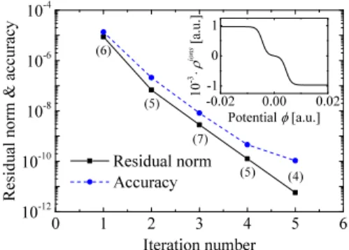
found that only a relatively small number of self-consistency iterations is needed in this approach to solve both the Poisson-Boltzmann and the modified Poisson-Poisson-Boltzmann problems. Fig. 4 shows the Euclidean norm of the residual vector rk
(black squares) and the accuracy of the numerical solution (blue circles) for the modified Poisson-Boltzmann solver with free boundary conditions. The solver exhibits a fast convergence, reaching an accuracy of∼10−10with some five
iterations. The inset shows ρions
[φ] as given by Eqs. (5) and(19), revealing an ionic density saturation in the solvent for electrostatic potentials whose absolute value is higher than ∼0.01 a.u. Numbers between round brackets represent the number of iterations needed to solve the GPe at step 4 of Algorithm 4 using the PCG scheme. The convergence criterion for the GPe solver has been fixed equal to the one of Algorithm4, except for the first two iterations where very accurate potentials do not change the overall performances of the PBe solver. Furthermore, its behavior does not change with the boundary conditions which are managed by means of the generalized Poisson solver. The latter also fixes the final accuracy of the self-consistent procedure. It is worth noting that performances and parallel efficiency as well as boundary conditions of both GPe and (M)PBe solvers are, eventually, delegated to the underlying SPe solver.
FIG. 4. Euclidean norm of the residual vectorrk (black squares) and
ac-curacy of the numerical solution (blue circles) for the modified Poisson-Boltzmann solver with free boundary conditions. Numbers between round brackets represent the number of iterations needed to solve the GPe at step 4 of Algorithm4. The inset showsρions[φ]given by Eqs.(5)and(19).
IV. ELECTRONIC-STRUCTURE COMPUTATIONS
Effects of complex wet environments surrounding an atomistic system can be approximately included into density functional calculations by simply introducing a dielectric cavity surrounding the atomistic system and taking in Eq.(1) the electrostatic potentialφ[ρ](r)as solution of the generalized Poisson or Poisson-Boltzmann equation. The PCG solver for the GPe (Algorithm2) has been implemented in the electronic-structure package BigDFT,25–28extending the capability of the code beyond vacuum-simulations.
Two distinct approaches have been implemented and tested to build up the dielectric cavity enveloping the atomic system. In both approaches, the cavity, mapped by the dielectric functionϵ(r), is fully differentiable and continuous in the whole simulation domain. In the first approach, the function ϵ(r) is defined starting from spherical-symmetric atom-centered cavities. Each sphere depends only on the radial distance with respect to a fixed atomic position. The whole rigid cavity is kept fixed during the whole SCF cycle in a DFT simulation.
On the other hand, it could be argued that regions occupied by atoms and their associated electronic charge density are strictly related. In other words, the actual value of the charge density might determine how much “space” is occupied by the solute. Starting from this idea, a cavity can be built up directly from the electronic density, as it has been shown in various publications.15,29,30 In this second approach, the dielectric function is not explicitly space-dependent, but can be implicitly mapped by means of the electronic charge density.
A. Rigid cavity
The most widespread continuum solvation model, which tries to include the effects of a surrounding dielectric medium in an implicit way, is the polarizable continuum model developed by Tomasi and co-workers.7,8,31 In the PCM formulation, the cavity surrounding the solute is sharp and discontinuous, and a polarization charge density is exactly localized at the vacuum-dielectric interface. In this way, the dielectric environment is represented by an effective surface polarization charge, reducing the three-dimensional dielectric problem into a two-dimensional one. Furthermore, the cavity can be considered rigid since it depends only on the atomic coordinates which does not vary during a SCF cycle in DFT simulations.
For a first test of the electrostatic solver integration (Algorithms1and2) in an electronic-structure code, a PCM-like cavity has been considered. The dielectric functionϵ(r) is thus given by the product of spherical-symmetric atom-centered error functions. Differently from the early PCM model, we here define a cavity which is fully differentiable and continuous. In particular, for a system of N atoms of coordinatesRi (fori=1, . . . ,N), the dielectric functionϵ(r)
can be expressed as
ϵ(r,{Ri})=(ϵ0−1)
i
h(di,∆;d(r,Ri))
+1, (23)
whereϵ0is the dielectric constant of the surrounding medium
and the function h is defined by Eq. (17). In Eq. (23)
d(r,Ri)=∥r−Ri∥, di are the cavity radii which depend
on the particular atom species, and ∆a parameter (kept fix for all atoms) which controls the transition region (≈4∆wide) from 0 to 1 where the polarization charge is located. Starting from Eq. (23), all vectors which explicitly depend on ϵ(r) can be analytically computed. The cavity is uniquely defined onceRi,di, and∆are fixed. All environment-dependent fields
are calculated once at the start of the solver and kept fixed throughout the procedure.
It has to be noticed that this definition of the cavity relies on the explicit dependence of ϵ(r,{Ri}) from the
atomic coordinates Ri (and, consequently, of the system
Hamiltonian). This dependence gives rise to additional terms when atomic forces are computed. The analytical rigid cavity above described should overcome this problem allowing a direct analytic calculation of such additional contributions. Furthermore, the values ofdiand of∆have to be tuned by the
user, usually by choosing a solvent-dependent scaling factor with respect to empirical Van der Waals radii.32A solution that would remove part of this arbitrariness should therefore avoid an explicit use of atomic coordinates in the cavity mapping. This will be the subject of Sec.IV B.
B. Charge-dependent cavity
For this definition of the cavity, the dielectric function does not explicitly depend in the atomic positions, but implicitly via the charge density ρelec,
ϵ(r)=ϵ[ρelec](r). (24)
This approach allows the cavity to self-consistently change during the SCF loop, strictly following the modifi-cation of the electronic charge density. A cavity surrounding an atomic system can be generated by means of two threshold parameter, i.e.,ρmaxandρmin, fixingϵ(r)=1 in regions when
ρelec(r)> ρmaxandϵ(r)=ϵ
0when ρelec(r)< ρmin. Like diin
the rigid case, ρmax fix the width of the cavity, whilst the extension of the transition region, previously defined by∆, is now tuned by ρmin.
Several features make the charge-dependent cavity more advantageous with respect to the rigid one. First, once the electron charge density is given, only two parameters uniquely define both the cavity and the transition region for the whole atomic system. Furthermore, since the dielectric function does not explicitly depend on the atomic coordinates, the evaluation of ionic forces can be done without modifications with respect to a simulation in gas-phase.
Among several ways to define the functional dependence on the electronic charge density, the self-consistent continuum
solvation (sccs) model developed in Ref. 15 has been
implemented. It allows to fit experimental solvation energies on a set of 240 neutral solutes with a mean absolute error of 1.2 kcal/mol,
ϵ(ρelec
)=
1 ρelec> ρmax
ϵw(ρelec)
0 ρmin< ρ
elec< ρmax
ϵ0 ρelec< ρmin
, (25)
where w(x) is a continuous smooth function describing the transition region between vacuum (where atoms are placed) and the full dielectric medium,
w(x)= 1
2π[z(x)−sin(z(x))], (26)
z(x)=2πln
ρmax
x
ln(ρmax
ρmin
). (27)
A good description of this region by means of Eq.(25) is mandatory for the procedure convergence as well as for the mapping of the polarization charge there confined. Since ϵ(r) explicitly depends on ρelec
(r), its variation needs to be included in the Kohn-Sham (KS) potential. Starting from Eq.(3) and integrating by parts, the electrostatic energy can be rewritten as
Ee s[ρ]=
1 2
ρφ[ρ]dr= 1 8π
ϵ[ρ](∇φ[ρ])2dr. (28)
Its functional derivative with respect toρgives the electrostatic potentialφ(r)plus an additional termvϵ(r),
vϵ(r)=− 1
8π dϵ(ρelec
(r)) dρelec |∇φ(r)|
2, (29)
which has to be added to the KS potential.
C. Solvation free energies
In order to test the integration and performances of the generalized Poisson solver into ab initio codes, the whole procedure previously described, i.e., Algorithms 1 and2 of Secs. II A and II B, rigid and charge-dependent cavities of Secs. IV A and IV B as well as the additional term of Eq.(29)have been integrated in the main BigDFT package.28 This extension allows to handle complex wet environments in electronic-structure calculations, including implicitly the effects of a solvent surrounding an atomic system.
The electrostatic solvation energy is defined as difference between the total energy of a given atomic system in the presence of the dielectric environment and the energy of the same system in vacuum
∆Gel=Gel−G0. (30)
A full comparison with experimental solvation energies needs the inclusion of non-electrostatic contributions. In this case, the main terms in the solute Hamiltonian, as introduced by PCM,8are
∆Gsol=∆Gel+Gcav+Grep+Gdis+Gt m+P∆V, (31)
where∆Gelis the electrostatic contribution,Gcavthe cavitation energy, i.e., the energy necessary to build up the solute cavity inside the solvent medium. Grep is a repulsion term representing the continuum counterpart of the short-range interactions induced by the Pauli exclusion principle, whilst Gdisreflects van der Waals interactions. The thermal termGt m
accounts for the vibrational and rotational changes and, finally, P∆V includes volume change in the solute Hamiltonian.
The inclusion of all non-electrostatic contributions goes beyond the aim of the present paper, where testing of the generalized Poisson solver and its integration into first
TABLE I. Electrostatic solvation energies∆Gel(in kcal/mol).
PCMa Rigid
BigDFT sccsPQEb sccsFBigDFT
NH3 −6.65 −6.28 −5.39 −5.35
H2O −8.98 −8.32 −8.21 −8.23
CH4 −0.61 −1.20 −0.68 −0.63
CH3OH −6.78 −6.57 −5.89 −5.83
CH3NH2 −4.51 −5.71 −4.53 −4.45
CH3CONH2 −12.53 −12.97 −11.87 −11.87
aPolarizable continuum model results obtained with
0936and Pauling’s set of atomic radii.34
bSelf-consistent continuum solvation model results from periodic BC calculations in
Ref.15.
principle atomistic calculations is the main goal. Therefore, only electrostatic solvation energies have been computed for a set of small neutral organic molecules.
Water has been chosen as solvent for all cases, with a dielectric constant of ϵ0=78.36 (experimental value at
low frequency and ambient conditions). Final energies for all molecules have been extracted after a full geometry optimization both in vacuum and in aqueous solution. In all cases, the surrounding dielectric medium lowers the total energy of the system with respect to vacuum, because the polarization of the dielectric stabilizes the solutes.
Table I reports electrostatic solvation energy ∆Gel obtained both with rigid and charge-dependent cavities under free boundary conditions. As previously stated, a critical point of PCM approaches is the choice of shape and size of the cavity, which should mimic the solute incorporating the whole atomic charge density. From its first formulation,31 PCM atomic radii Ri were fixed proportional to the van der
Waals radii,Ri= f ·RivdW. In our rigid model, a proportional
factor of f =1.2 has been fixed and the Pauling’s set of atomic radii has been considered33–35(except for the hydrogen atoms bound to heteroatoms which have a radius value of 1 Å). Having a further degree of freedom with respect to sharp PCM cavities, a∆=0.5 a.u. has been tuned and kept constant for all atoms.
As reference, in Table I, PCM calculations together with sccs calculations from Ref. 15 have been reported. The first were performed with the 09 code,36
but using the version of PCM which was the default in 03, as specified by the keyword g03defaults. Only electrostatic solvation effects were included in the calculation and, to simplify the comparison, the simple van der Waals surface was adopted with Pauling’s set of atomic radii34(explicit hydrogens), but without the additional smoothing used to describe the solvent-excluded surface. The Perdew-Berke-Ernzerhof (PBE) functional37 and the extended triple-zeta 6-311+g(d,p) basis set were used for both geometry optimizations and energy calculations, in vacuum and in solution, consistently with the setup used for the parameterization of the electrostatic solvation energy in sccs.15
In all calculations, soft norm-conserving pseudopotentials including non-linear core correction38,39 along with PBE functional were used to describe the core electrons and exchange-correlation, respectively.
FIG. 5. Accuracy of the Kohn-Sham total energy with respect to the spatial gridhgrid. Calculations for all molecules have been done both in vacuum (empty symbols, dashed lines) and with a surrounding dielectric environment (filled symbols, solid lines) in free boundary conditions.
For the charge-dependent cavity, values ofρmax=5·10−3
a.u. and ρmin=1·10−4a.u. have been fixed which produce a
mean absolute error of 1.20 kcal/mol for the solvation energies of a database of 240 molecules.15 A perfect agreement has been reached which confirms the performance and reliability of the integrated generalized Poisson solver.
In order to test and validate the whole electrochemical library in BigDFT, the effects of grid resolution and boundary conditions on the electrostatic solvation energies for the same set of neutral molecules have been investigated. The global accuracy is strictly related to the size of the simulation box and the spatial grid resolutionhgrid. However, a decrease of the
latter can affect the whole cost of the calculation both in time and memory usage. Consequently, it is worth to investigate the effects of the dielectric medium’s inclusion in a DFT run with respect to the vacuum case.
In that respect, Kohn-Sham total energies have been extracted both in vacuum and in the presence of the solvent (water) as function of the spatial grid hgrid. Its accuracy
is reported in Fig. 5 as difference with the reference value at hgrid=0.20 bohr. Results show that the accuracy
is not affected by the surrounding dielectric environment (filled symbols, solid lines) with respect to the vacuum case (empty symbols, dashed lines). Following the same guidelines, the accuracy of the electrostatic solvation energy [Eq. (30)] with respect to the spatial grid hgrid has been
investigated and reported in Fig.6. Results indicate that anhgrid =0.30 bohr in BigDFT with free boundary condition provides electrostatic solvation energies with an accuracy lower than ∼10−2kcal/mol.
Since isolated systems embedded in a wet environment are the subject of interest, spurious long range electrostatic interactions with periodic images due to artificially imposed periodicities along certain direction can be problematic. In the developed procedure, the boundary conditions enter through the preconditioner, i.e., the SPe solver. Since in the BigDFT Poisson solver, all the common boundary conditions such as free, wire, and surface are exactly implemented, such spurious interactions do not exist at any stage of our approach.
FIG. 6. Accuracy of the electrostatic solvation energy with respect to the spatial gridhgridwith free boundary conditions.
Fig. 7 reports the difference between the electrostatic solvation energies computed with periodic and free boundary conditions as function of the periodic cell length and keeping fixed the spatial grid hgrid=0.20 bohr. Molecules have been
ordered according to the strength of their electrostatic dipole, from largest to smallest. Dipole values for each molecule are reported in Table IIboth in vacuum and in the presence of a water solvent. It can be noticed that the presence of the polar solvent increases the electrostatic dipoles of the molecules.32 As it might be expected, the free BC calculation represents the asymptotic result for periodic BC run of increasing box sizes. Interactions with image-molecules are less relevant for molecules with small dipole moment like CH4, but are
not negligible for molecules with larger dipoles such as CH3CONH2. In such cases unrealistic large periodic boxes
are required for periodic BC to reproduce the free boundary condition results with high accuracy.
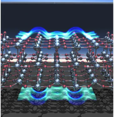
Numerous processes of practical interest involve surfaces in contact with neutral or ionic solvents, leading to an induced polarization charge on the dielectric medium or an electric double layer. The BigDFT package allows to use exact surface boundary conditions avoiding spurious interaction in the direction orthogonal to the surface. To show a further application of the solvation library in BigDFT, a TiO2surface
in contact with pure water has been simulated. The full DFT simulation in presence of the solvent has been initialized starting from its relaxed state in vacuum. Fig. 8 shows the
FIG. 7. Difference between the electrostatic solvation energy computed with periodic and free boundary conditions as a function of the periodic cell length. Molecules have been ordered as a function of their electrostatic dipole norm, from largest to smallest (see TableII).
TABLE II. Molecule dipole norm in vacuum and water solvent (in Debye).
Dipolevacuum Dipolewater
CH3CONH2 3.88 5.76
H2O 1.81 2.41
CH3OH 1.57 2.14
NH3 1.49 1.98
CH3NH2 1.27 1.78
CH4 0.00 0.00
TiO2 wet surface as well as isosurfaces of the polarization
charge density ρpol as given by Eq. (10). In this test case, an electrostatic solvation energy of−46.60 kcal/mol has been recovered for the TiO2 slab in contact with the dielectric
medium.
D. Performances for a full SCF run
In this section, we report the performances of an entire electronic-structure calculation using the extended BigDFT package containing our new Poisson solver applied to non-vacuum environments. As a test system, we took the protein PDB ID: 1y49 (122 atoms), which was also chosen as a benchmark system in another recent publication on an optimized version of the COSMO40 Poisson solver for dielectric environments.41The approach in this publication is quite different from ours. A small Gaussian type basis set was used, whereas we use a systematic basis set of wavelets. Also
FIG. 8. TiO2surface in contact with water: Isosurfaces of the polarization chargeρpolin the implicit dielectric medium.
the hardware targeted was different. We target traditional massively parallel supercomputers, whereas they targeted powerful single nodes that were enhanced with graphics processing unit (GPU) hardware. In spite of all the differences we will see that in both approaches, the overhead for a simulation in a dielectric medium compared to vacuum is rather small and that the total numerical effort is also quite similar. In our tests, the rigid PCM-like cavity has been used together with the parameter’s setting of Sec. IV C and a spatial gridhgrid=0.40 bohr. The direct minimization method
of BigDFT25for the calculation of the converged wavefunction was used.
Both the developed preconditioned conjugate gradient and the self-consistent algorithm have been applied for the electrostatic problem (generalized Poisson equation) with and without the use of an input guess from previous routine calls. As accurate potentials are not needed during the first stages of the SCF wavefunction optimization loop, a dynamic exit threshold from Algorithms 1 and 2 based on the norm of the residual vector rk has been implemented. It is allowed
to vary between τmin and τgnrm, where the last is the norm
of the KS energy gradient from the previous wavefunction SCF iteration. Aτmin=10−4guarantees a correct SCF
conver-gence while lowering the overall electrostatic calculation time.
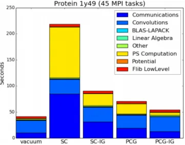
The whole electrochemical library, namely, the general-ized Poisson and the Poisson-Boltzmann solvers, has been fully embedded in the parallelization scheme of BigDFT, which exploits two levels of parallelization, i.e., MPI and OpenMP. For our test system, which has 179 orbitals, 45 MPI tasks with 4 OpenMP threads were used. The simulations were performed on a Cray XC30 system whose nodes are equipped with 8-core 64-bit Intel SandyBridge CPU (Intel® Xeon®
E5-2670) and NVIDIA® Tesla® K20X. Fig. 9 reports a
detailed schematic of timings for the total SCF convergence of BigDFT runs both in gas phase and with the inclusion of the
FIG. 9. Relative timings for full SCF convergence in a BigDFT run for a solvated 1y49 protein (122 atoms). Each column refers to a particular algorithm (SC and PCG) to handle the generalized Poisson equation (IG means the use of input guess). Colors indicate the load of the different run categories. SCF vacuum data are also reported for comparison. Absolute timings are reported in TableIII.
TABLE III. BigDFT timings and performances for 1y49 protein.
Algorithm Environment
SCF loop (s)
GP solver (s)
Total GPe iterations
No. of SCF iterations
Vacuum solver
Vacuum 42 0.43 1 16
SC Water 218 97 342 18
SC-IG Water 91 23 60 18
PCG Water 71 19 686 16
PCG-IG Water 54 5.50 178 18
implicit solvent. Each column refers to a particular algorithm (SC and PCG) to solve the generalized Poisson equation (IG means the use of input guess). Colors indicate the load of the different timing categories. SCF vacuum data are also reported for comparison.
Fig.9shows the relative cost to include implicit solvent-solute interactions with respect to its gas phase using our generalized Poisson solver. These additional efforts can be visualized by the yellow and dark blue blocks which are related, respectively, to the electrostatic solver and communications. The ratio of the wavefunction optimization runtime in solvent and gas phase strongly varies with respect to the algorithm chosen. Using an input guess from the previous calculation strongly decreases the computational runtime for both approaches (PCG and SC). However, the best performances come out for the PCG algorithm with input guess (PCG-IG) where a ratio of 1.28 is recovered. So thanks to the PCG algorithm, which requires only vacuum Poisson solver calls and fully parallelizable operations (without the use of finite-difference filters like in the SC algorithm), a small overhead for the solvent calculation can be obtained. Similar performance ratios are also found for runs of the same system on a single node of the above mentioned machine, with 8 OpenMP threads, where a vacuum run takes 741 s and a PCG-IG run needed 857 s, i.e., only about 15% slower.
Table III reports run data for all single-point energy evaluations of Fig. 9. It shows the total time spent in the SCF wavefunction optimization loop, the time spent in the electrostatic solver, the sum of all generalized Poisson iterations during the whole SCF loop, and the number of SCF iterations needed to converge both for vacuum and the implicit solvent case.
V. CONCLUSIONS
In the present work, a library to handle complex wet-environments in electronic-structure calculations has been presented. It allows to include on the atomistic scale effects of an aqueous environment in an implicit way. The solver is able to handle both the generalized Poisson and several variants of the Poisson-Boltzmann equation. The core of the generalized Poisson solver is a preconditioned conjugate gradient algorithm which allows to numerically solve the minimization problem with some ten iterations. The same algorithm works for the linear case of the Poisson-Boltzmann
equation, whilst for the general case, a self-consistent procedure has been implemented. The chosen preconditioner is based on the ISF Poisson solver for the standard Poisson equation, which can handle all common boundary conditions exactly. The code requires a small amount of memory and is very fast and in addition also highly parallelized. We have shown that coupled with BigDFT, our method can correctly reproduce electrostatic solvation energies of a set of small neutral organic molecules. Effects of grid resolution and boundary conditions on the electrostatic solvation energies have been also reported. The whole library will be released as an independent program suitable for integration in other electronic structure codes. A GPU-accelerated version of this software package is also in preparation, following the guidelines indicated in Ref.42.
ACKNOWLEDGMENTS
This work was done within the PASC and NCCR MARVEL projects. Computer resources were provided by the Swiss National Supercomputing Centre (CSCS) under Project ID s499. L.G. acknowledges also support from the EXTMOS EU project.
1I. Dabo, Y. Li, N. Bonnet, and N. Marzari, “Ab initioelectrochemical
prop-erties of electrode surfaces,” inFuel Cell Science: Theory, Fundamentals and Bio-Catalysis, edited by A. Wieckowski and J. Nørskov (John Wiley & Sons, Inc., 2010), pp. 415–431.
2C. Reichardt,Solvents and Solvent Effects in Organic Chemistry, 3rd ed.
(WILEY-VCH, Weinheim, 2003).
3J. A. White, E. Schwegler, G. Galli, and F. Gygi,J. Chem. Phys.113, 4668 (2000).
4S. Goedecker,J. Chem. Phys.120, 9911 (2004).
5B. Schaefer, S. Mohr, M. Amsler, and S. Goedecker,J. Chem. Phys.140, 214102 (2014).
6L. Onsager,J. Am. Chem. Soc.58, 1486 (1936). 7J. Tomasi and M. Persico,Chem. Rev.94, 2027 (1994).
8J. Tomasi, B. Mennucci, and R. Cammi,Chem. Rev.105, 2999 (2005). 9C. J. Cramer and D. G. Truhlar,Chem. Rev.99, 2161 (1999). 10L. Greengard and V. Rokhlin,J. Comput. Phys.73, 325 (1987). 11M. C. Strain, G. E. Scuseria, and M. J. Frisch,Science271, 51 (1996). 12L. Genovese, T. Deutsch, A. Neelov, S. Goedecker, and G. Beylkin,J. Chem.
Phys.125, 074105 (2006).
13L. Genovese, T. Deutsch, and S. Goedecker,J. Chem. Phys.127, 054704 (2007).
14A. Cerioni, L. Genovese, A. Mirone, and V. A. Sole,J. Chem. Phys.137, 134108 (2012).
15O. Andreussi, I. Dabo, and N. Marzari, J. Chem. Phys. 136, 064102 (2012).
16J.-L. Fattebert and F. Gygi,Int. J. Quantum Chem.93, 139 (2003). 17M. Gouy,J. Phys. Theor. Appl.9, 457 (1910).
18D. L. Chapman,Philos. Mag.25, 475 (1913).
19O. Stern, Z. Electrochem.30, 508 (1924), http://chemport.cas.org/cgi-bin/
sdcgi?APP=ftslink&action=reflink&origin=ACS&version=1.0&coi=1%3 ACAS%3A528%3ADyaB2MXls1Wh&md5=0bb6a0352af08f94aa161e9c 561d8784.
20J. Bikerman,Philos. Mag.33, 384 (1942).
21M. Otani and O. Sugino,Phys. Rev. B73, 115407 (2006). 22R. Jinnouchi and A. B. Anderson,Phys. Rev. B77, 245417 (2008). 23I. Dabo, “Towards first-principles electrochemistry,” Ph.D. thesis, MIT,
Cambridge, MA (2008).
24J. J. López-García, J. Horno, and C. Grosse,Langmuir27, 13970 (2011). 25L. Genovese, A. Neelov, S. Goedecker, T. Deutsch, S. A. Ghasemi, A.
Wil-land, D. Caliste, O. Zilberberg, M. Rayson, A. Bergman, and R. Schneider,
J. Chem. Phys.129, 014109 (2008).
26L. Genovese, B. Videau, M. Ospici, T. Deutsch, S. Goedecker, and J.-F.
Mhaut,C. R. Mec.339, 149 (2011).
27S. Mohr, L. E. Ratcliff, P. Boulanger, L. Genovese, D. Caliste, T. Deutsch,
and S. Goedecker,J. Chem. Phys.140, 204110 (2014). 28BigDFT code website,www.bigdft.org.
29J.-L. Fattebert and F. Gygi,J. Comput. Chem.23, 662 (2002).
30D. A. Scherlis, J.-L. Fattebert, F. Gygi, M. Cococcioni, and N. Marzari,
J. Chem. Phys.124, 074103 (2006).
31S. Miertuš, E. Scrocco, and J. Tomasi,Chem. Phys.55, 117 (1981). 32M. Orozco and F. J. Luque,Chem. Rev.100, 4187 (2000).
33T. Mineva, N. Russo, and E. Sicilia,J. Comput. Chem.19, 290 (1998). 34L. Pauling,The Nature of the Chemical Bond, 3rd ed. (Cornell University
Press, Ithaca, NY, 1960).
35CRC Handbook of Chemistry and Physics, 96th edition, electronic release,
2015-2016,www.hbcpnetbase.com.
36M. J. Frisch, G. W. Trucks, H. B. Schlegelet al.,
09, RA.1, G, I., W, CT, 2009 .
37J. P. Perdew, K. Burke, and M. Ernzerhof,Phys. Rev. Lett.77, 3865 (1996). 38S. Goedecker, M. Teter, and J. Hutter,Phys. Rev. B54, 1703 (1996). 39A. Willand, Y. O. Kvashnin, L. Genovese, l. Vázquez-Mayagoitia, A. K.
Deb, A. Sadeghi, T. Deutsch, and S. Goedecker,J. Chem. Phys.138, 104109 (2013).
40A. Klamt and G. Schuurmann,J. Chem. Soc., Perkin Trans.2, 799 (1993). 41F. Liu, N. Luehr, H. J. Kulik, and T. J. Martínez,J. Chem. Theory Comput.
11, 3131 (2015).
42N. Dugan, L. Genovese, and S. Goedecker,Comput. Phys. Commun.184, 1815 (2013).